Code
library(ggplot2)
map_file <- "data/pigment_snp_map.tsv"
have_map <- file.exists(map_file)What SNPs SEPIA analyzes, where each came from, and how confident we are in it
Lily’s thesis (PAINT) analyzed a fixed 222-SNP pigmentation panel pulled from the GWAS Catalog. SEPIA’s bigger question needs more than that: the pigmentation-gene-network project assembles the pigmentation literature into a much larger, multi-source SNP set. This page is the auditable record of exactly which SNPs we carry, where each one came from, how we put them on a single coordinate system, and — importantly — how confident we are in each, because a raw GWAS-Catalog pull mixes strongly-replicated loci with single-study, unreplicated hits.
Everything here is generated from data/pigment_snp_map.tsv, which is built by code/build_pigment_snp_map.py (re-resolving every rsID to both genome builds via Ensembl). The 222-panel subset is preserved and flagged, so this strictly extends Lily’s work rather than replacing it.
library(ggplot2)
map_file <- "data/pigment_snp_map.tsv"
have_map <- file.exists(map_file)m <- read.delim(map_file, stringsAsFactors = FALSE)
n_total <- nrow(m)
n_panel <- sum(m$in_222_panel == "yes", na.rm = TRUE)
n_new <- n_total - n_panel
n_ok <- sum(m$status == "ok", na.rm = TRUE)Each SNP is drawn from one or more rsID-bearing pigmentation sources, then re-resolved to verified coordinates. Coordinates in the source files are mixed-build and inconsistent (GWAS Catalog rows are hg38; the case-study extractions are hg19; HIrisPlex-S has no coordinates at all), so we do not trust any of them — we re-pull each rsID’s GRCh38 and GRCh37 position + alleles from Ensembl, keyed by rsID. (This is the same approach that caught the +1 off-by-one in the original panel’s hg38 coordinates.) We flag palindromic SNPs (A/T, C/G — strand-ambiguous), multiallelic sites, and merged rsIDs.
# one SNP can have several sources; count membership per source tag family
fam <- function(s) {
  s <- strsplit(s, ";")[[1]]
  s <- ifelse(grepl("^curated:", s), "curated_paper", s)
  unique(s)
}
src_tab <- sort(table(unlist(lapply(m$sources, fam))), decreasing = TRUE)
knitr::kable(data.frame(source = names(src_tab), n_SNPs = as.integer(src_tab)),
caption = "SNPs contributed by each source (a SNP can appear in more than one).")| source | n_SNPs |
|---|---|
| gwas_catalog | 1072 |
| curated_paper | 69 |
| martin2017 | 49 |
| discordance | 48 |
| hirisplex_s | 36 |
| kim2024 | 26 |
What each source is:
The user-facing distinction the raw catalog can’t make on its own: replicated vs not. We assign each SNP a confidence tier as the best evidence across its sources:
gwas_replicated/gwas_n_assoc ≥ 2), or a HIrisPlex-S validated marker, or a genome-wide-significant Martin/Kim lead SNP.m$confidence <- factor(m$confidence, levels = c("high","moderate","low"))
tab <- as.data.frame(table(confidence = m$confidence,
set = ifelse(m$in_222_panel == "yes", "in 222-panel", "new to SEPIA")))
ggplot(tab, aes(confidence, Freq, fill = set)) +
geom_col(position = "dodge") +
geom_text(aes(label = Freq), position = position_dodge(0.9), vjust = -0.3, size = 3) +
scale_fill_manual(values = c("in 222-panel" = "#4C6EF5", "new to SEPIA" = "#E4572E"), name = NULL) +
labs(title = "Pigmentation SNPs by confidence tier",
subtitle = "high = replicated / forensically validated · low = single unreplicated GWAS hit",
x = NULL, y = "SNPs") +
theme_minimal(base_size = 12) + theme(panel.grid.major.x = element_blank())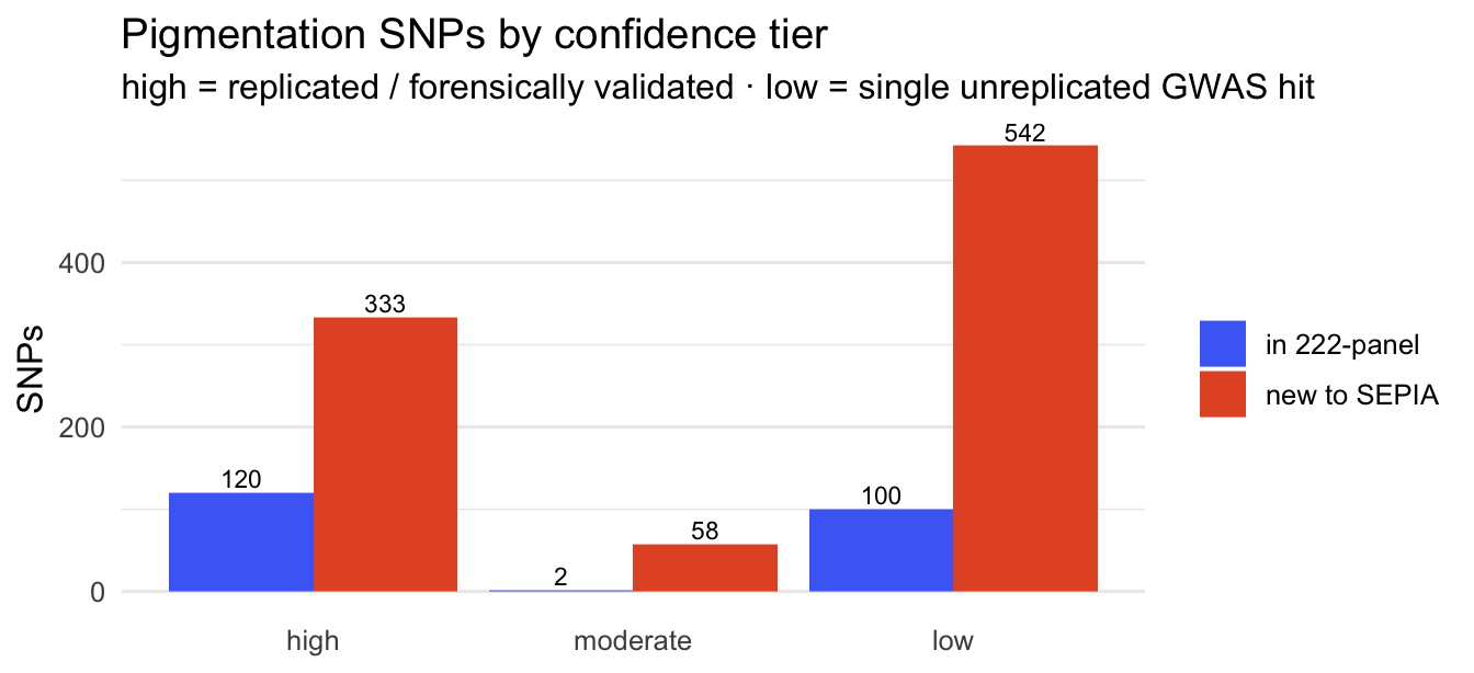
knitr::kable(data.frame(
  metric = c("Total SNPs", "In the original 222-panel", "New to SEPIA",
             "High confidence", "Moderate", "Low (single unreplicated GWAS)",
             "Palindromic (flagged for Q4)", "Merged rsIDs", "Resolved on both builds"),
  count  = c(n_total, n_panel, n_new,
             sum(m$confidence == "high"), sum(m$confidence == "moderate"), sum(m$confidence == "low"),
             sum(m$palindromic == "yes", na.rm = TRUE), sum(m$merged == "yes", na.rm = TRUE), n_ok)),
caption = "SNP-set summary (generated from data/pigment_snp_map.tsv).")| metric | count |
|---|---|
| Total SNPs | 1155 |
| In the original 222-panel | 222 |
| New to SEPIA | 933 |
| High confidence | 453 |
| Moderate | 60 |
| Low (single unreplicated GWAS) | 642 |
| Palindromic (flagged for Q4) | 213 |
| Merged rsIDs | 5 |
| Resolved on both builds | 1153 |
ok SNP here (correct hg19 coordinates), replacing the 222-SNP panel — and we can re-run it high-confidence-only vs all to see how much the unreplicated tail moves the result.The gene-network’s gene-level tables — Bajpai (CRISPR hits), Baxter (curated genes), Raghunath (melanogenesis network), D’Arcy (disease genes / PPI) — are gene-symbol-only, no SNP coordinates. Using them requires a separate gene→coordinate join (items B6/B7) and they never enter the SNP-level PCA or scores. They are deferred by decision, not oversight.