---
title: "Modern reference panel PCA (SGDP)"
subtitle: "Quality control: does the modern reference recover global human structure?"
---
## Why this check comes first
Before SEPIA compares any archaic genome to modern humans, we check that the
**modern reference behaves sensibly on its own**. If the modern samples don't
separate into the broad geographic groups we expect, nothing built on top of them
(projecting archaics, reading pigmentation loci) can be trusted.
There is a concrete reason to check. The modern reference SEPIA inherited was an
**incomplete merge — only 15 of the 166** available Simons Genome Diversity Project
(SGDP) individuals. Fifteen genomes cannot define global structure, and the symptom
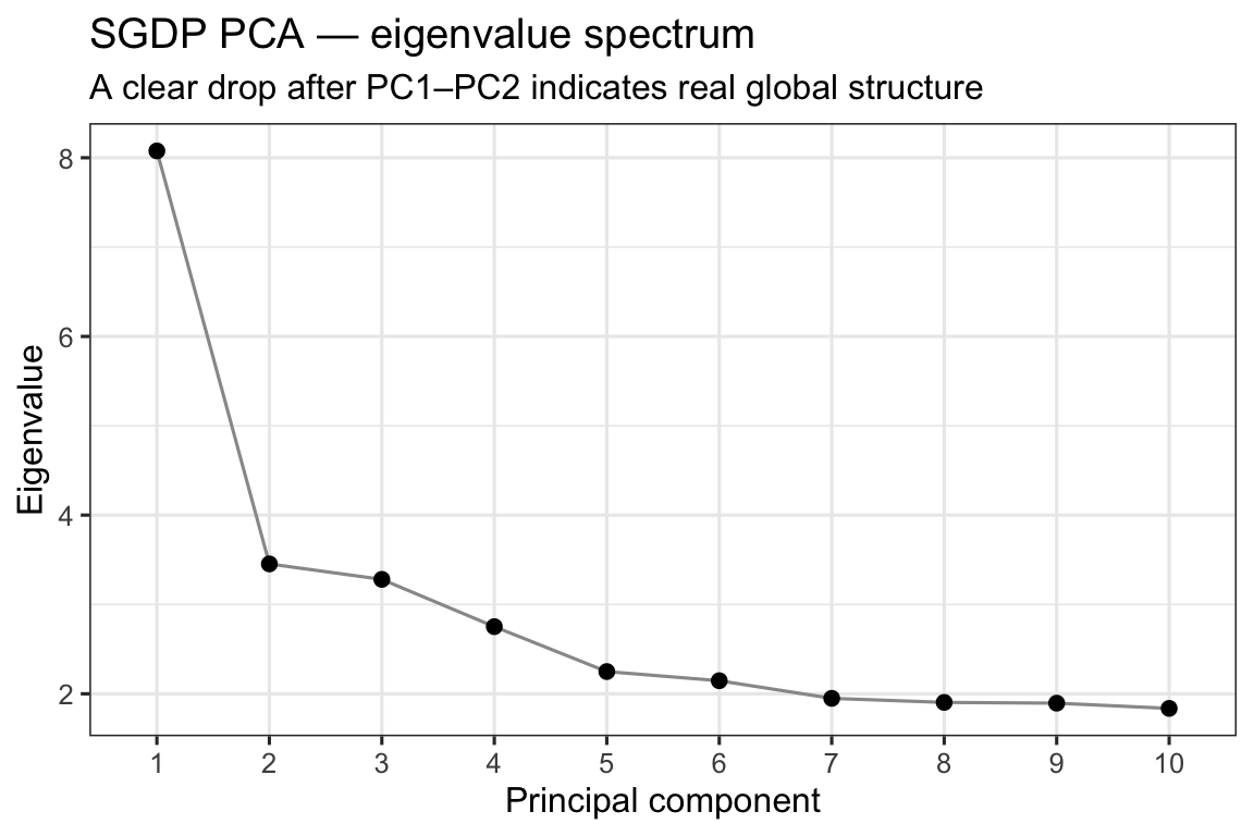
was a near-degenerate PCA (the eigenvalues after PC1 were essentially flat — see the
[bug-evidence log](plan/verify/BUG_EVIDENCE.html)). We rebuilt the reference from
**all 166** individuals. This page is the check: with the full set, do the modern
samples spread into real structure, and is there a clear drop in the eigenvalue
spectrum rather than noise?
## What produced these inputs
Run on Great Lakes by [`code/wg_modern_merge.slurm`](https://github.com/lasisilab/sepia/blob/main/code/wg_modern_merge.slurm):
`bcftools merge` of the 166 per-sample SGDP BCFs → PLINK (variant IDs set to
`chr:pos:ref:alt`, biallelic SNPs only) → LD-prune (`--indep-pairwise 200 25 0.4`) →
`plink2 --pca 10 allele-wts`. The reusable reference lands in the shared lab genomes
directory; the small PCA coordinates land in `output/pca_wg/` (tracked in this repo,
so this page renders from them).
```{r setup, message=FALSE, warning=FALSE}
library(ggplot2)
eig_file <- "output/pca_wg/sgdp166_pca.eigenvec"
val_file <- "output/pca_wg/sgdp166_pca.eigenval"
meta_file <- "data/sgdp_metadata.tsv"          # optional: IID -> region/population labels
have_pca <- file.exists(eig_file) && file.exists(val_file)
```
```{r not-ready, eval=!have_pca, echo=FALSE, results='asis'}
cat("::: {.callout-note}\n",
"**Not yet rendered with data.** Submit `code/wg_modern_merge.slurm` on Great Lakes; ",
"it writes `output/pca_wg/sgdp166_pca.eigenvec` and `.eigenval`. Re-render this page ",
"(`quarto render sgdp_reference_pca.qmd`) and the scree + PCA plots below will appear.\n:::\n",
sep = "")
```
## Is there real structure? (eigenvalue scree)
A healthy global PCA drops sharply after the first few PCs. The old 15-sample
reference did not — its spectrum was flat, a hallmark of too few samples / no
structure. We want to see a clear elbow here.
```{r scree, eval=have_pca, fig.width=6, fig.height=4}
val <- scan(val_file, quiet = TRUE)
scree <- data.frame(PC = factor(seq_along(val)), eigenvalue = val)
ggplot(scree, aes(PC, eigenvalue, group = 1)) +
  geom_line(colour = "grey60") + geom_point(size = 2) +
  labs(x = "Principal component", y = "Eigenvalue",
       title = "SGDP PCA — eigenvalue spectrum",
       subtitle = "A clear drop after PC1–PC2 indicates real global structure") +
  theme_bw(base_size = 12)
```
## Old vs. new reference
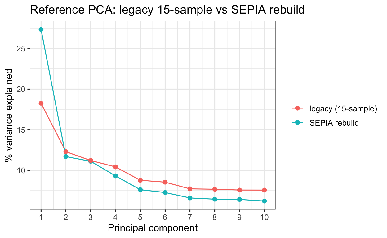
Direct before/after: the inherited reference had only 15 individuals; the SEPIA rebuild
uses the full set (159 after dropping truncated downloads). Overlaid as **% variance
explained** per PC (so the different sample counts are comparable), a rebuild that
recovered real structure should concentrate more variance in the leading PCs, whereas the
15-sample spectrum stays flat.
```{r compare, eval=have_pca, fig.width=6.5, fig.height=4}
old_file <- "data/sgdp.wg.pca.eigenval"          # legacy 15-sample modern PCA (committed)
mk <- function(f, label) { v <- scan(f, quiet = TRUE); data.frame(PC = seq_along(v), pct = 100 * v / sum(v), set = label) }
df <- mk(val_file, "SEPIA rebuild")
if (file.exists(old_file)) df <- rbind(df, mk(old_file, "legacy (15-sample)"))
ggplot(df, aes(PC, pct, colour = set)) +
  geom_line() + geom_point(size = 2) +
  scale_x_continuous(breaks = 1:10) +
  labs(x = "Principal component", y = "% variance explained", colour = NULL,
       title = "Reference PCA: legacy 15-sample vs SEPIA rebuild") +
  theme_bw(base_size = 12)
```
## Where does everyone land? (PC1 vs PC2)
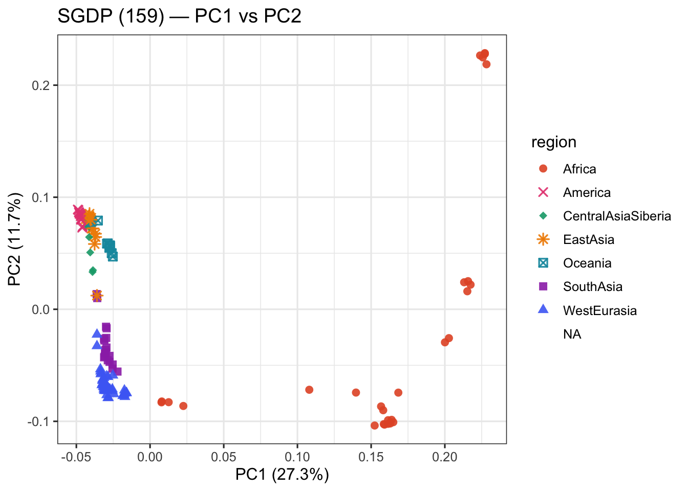
If the reference is sound, the samples should fan out into the broad continental
groups. We colour by region when SGDP metadata is available; otherwise points are
shown uncoloured (structure should still be visible as separated clouds).
```{r pca, eval=have_pca, fig.width=7, fig.height=5}
ev <- read.table(eig_file, header = FALSE, skip = 1, stringsAsFactors = FALSE)
names(ev) <- c("FID", "IID", paste0("PC", seq_len(ncol(ev) - 2)))

col_by <- NULL
if (file.exists(meta_file)) {
  meta <- read.delim(meta_file, stringsAsFactors = FALSE)
  ev <- merge(ev, meta, by = "IID", all.x = TRUE)
  col_by <- intersect(c("region", "population"), names(meta))[1]
}

source("plan/figures/_pca_style.R")
pc_var <- round(100 * val[1:2] / sum(val), 1)
p <- ggplot(ev, aes(PC1, PC2)) +
  labs(x = sprintf("PC1 (%.1f%%)", pc_var[1]),
       y = sprintf("PC2 (%.1f%%)", pc_var[2]),
       title = "SGDP (159) — PC1 vs PC2") +
  theme_bw(base_size = 12)
if (!is.null(col_by) && col_by == "region" && !all(is.na(ev$region))) {
  ev$region <- region_factor(ifelse(is.na(ev$region), "unknown", ev$region))
  p <- p + geom_point(aes(colour = region, shape = region), size = 2.2, stroke = 0.9, alpha = 0.9) +
    region_scales("region")
} else if (!is.null(col_by) && !all(is.na(ev[[col_by]]))) {
  p <- p + geom_point(aes(colour = .data[[col_by]]), size = 2, alpha = 0.9) + labs(colour = col_by)
} else {
  p <- p + geom_point(size = 2, alpha = 0.9, colour = "#1E5A54") +
    labs(caption = "No SGDP region labels found — points uncoloured.")
}
p
```
## Reading the result
- **Eigenvalue elbow present** → the reference carries real structure (the 15-sample
problem is fixed). A still-flat spectrum would mean the merge didn't actually add
diversity — investigate before going further.
- **Continental separation on PC1/PC2** (Africa vs the rest, then finer structure) →
the modern panel is trustworthy to project archaics onto (the archaic-projection step).
- Add the region colouring by dropping an SGDP `IID → region/population` table at
`data/sgdp_metadata.tsv` (public SGDP metadata; small).
Next: **the archaic-projection QC (next)** projects the archaic genomes onto this PCA (with
`no-mean-imputation`) to see whether they fall out as a sensible outgroup.