library(tidyverse)
library(ggrepel)
library(scales)
library(patchwork)
library(here)
library(lubridate)
library(qualpalr)
# Load literature data
literature_data <- read_csv(here("data", "ndis_crossref", "literature_data.csv"), show_col_types = FALSE) |>
mutate(asof_date = as.Date(asof_date))
# Get yearly aggregates from Python via reticulate
# Convert pandas DataFrame to R data.frame
py_df <- py$growth_data_yearly
growth_data <- data.frame(
year = as.numeric(py_df$year$values),
offender_profiles = as.numeric(py_df$offender_profiles$values),
arrestee = as.numeric(py_df$arrestee$values),
forensic_profiles = as.numeric(py_df$forensic_profiles$values),
investigations_aided = as.numeric(py_df$investigations_aided$values),
ndis_labs = as.numeric(py_df$ndis_labs$values),
total_profiles = as.numeric(py_df$total_profiles$values)
) |>
mutate(date = as.Date(paste0(year, "-06-01")))
# Define qualpal colors (matching manuscript_figures.qmd)
qualpal_palette <- qualpal(
n = 10,
list(
h = c(190, 330),
s = c(0.35, 0.75),
l = c(0.45, 0.85)
)
)
qp_hex <- qualpal_palette$hex
offender_color <- qp_hex[1]
arrestee_color <- qp_hex[3]
forensic_color <- qp_hex[4]
total_color <- qp_hex[5]
investigations_color <- qp_hex[6]
# Extended date range for consistent x-axis
extended_date_range <- c(
min(growth_data$date) - years(1),
max(growth_data$date) + years(1)
)
# Axis formatter
scale_axis <- function(values) {
ifelse(values >= 1e6, paste0(values / 1e6, "M"),
ifelse(values >= 1e3, paste0(values / 1e3, "K"), values))
}
label_size <- 10 / .pt
# Common theme
theme_crossref <- theme_minimal(base_size = 11) +
theme(
plot.title = element_text(face = "bold", size = 13),
panel.grid.minor = element_blank(),
panel.grid.major.x = element_blank(),
panel.grid.major.y = element_line(color = "gray90", linewidth = 0.3),
axis.line = element_line(color = "black", linewidth = 0.3),
axis.ticks = element_line(color = "black", linewidth = 0.3),
axis.text = element_text(color = "black", size = 10),
axis.text.x = element_text(angle = 45, hjust = 1),
legend.position = "none"
)
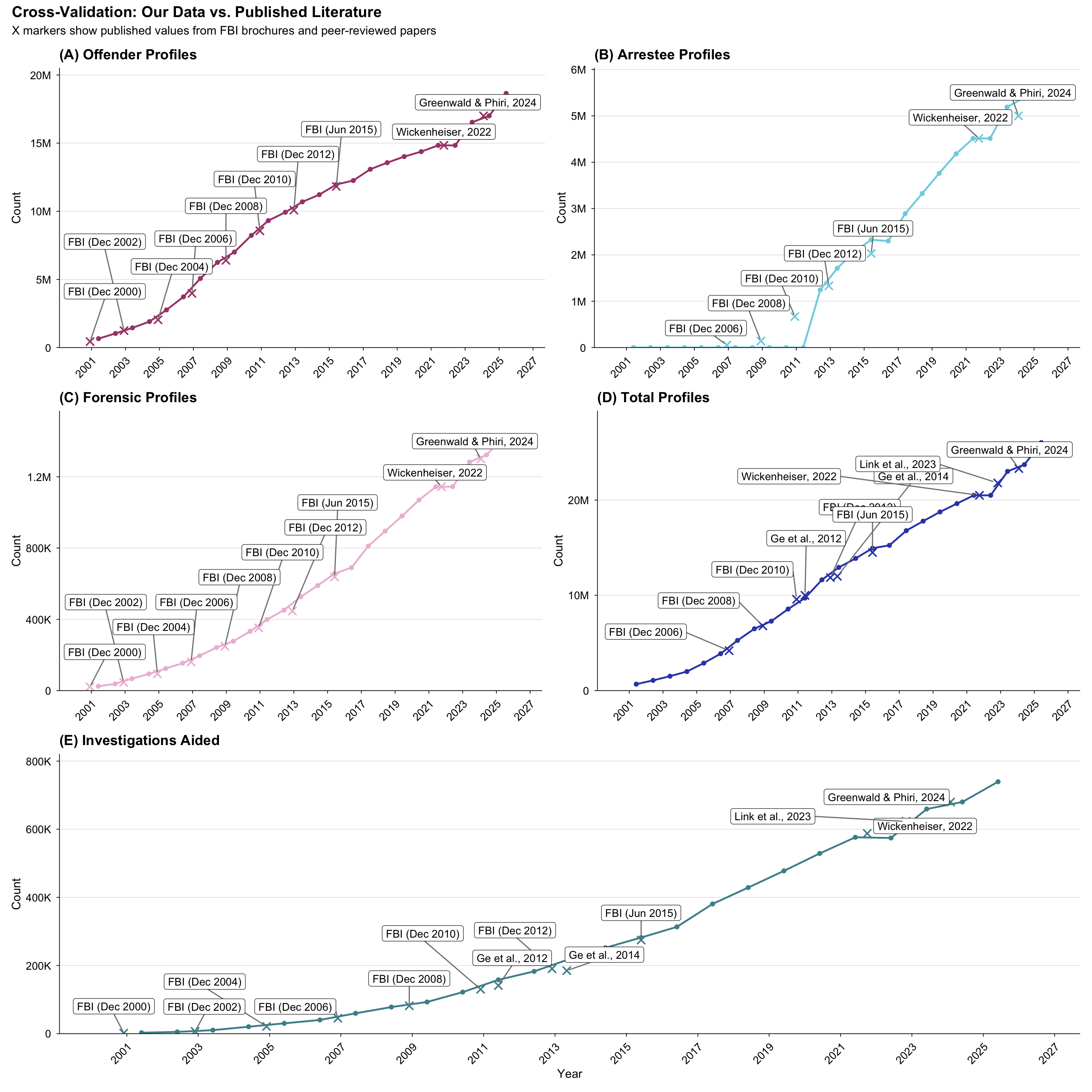
# 1. Offender Profiles
offender_lit <- filter(literature_data, !is.na(offender_profiles))
p1 <- ggplot() +
geom_line(data = growth_data, aes(x = date, y = offender_profiles),
color = offender_color, linewidth = 0.8) +
geom_point(data = growth_data, aes(x = date, y = offender_profiles),
color = offender_color, size = 1.5) +
geom_point(data = offender_lit, aes(x = asof_date, y = offender_profiles),
shape = 4, size = 2.5, stroke = 1, color = offender_color) +
geom_label_repel(
data = filter(offender_lit, year(asof_date) < 2020),
aes(x = asof_date, y = offender_profiles, label = short_label),
size = label_size, nudge_y = 4e6,
box.padding = 0.3, point.padding = 0.3, min.segment.length = 0.3,
segment.color = "gray50", max.overlaps = Inf,
fill = "white", label.size = 0.2
) +
geom_label_repel(
data = filter(offender_lit, year(asof_date) >= 2020),
aes(x = asof_date, y = offender_profiles, label = short_label),
size = label_size, nudge_y = 1e6,
box.padding = 0.3, point.padding = 0.3, min.segment.length = 0.3,
segment.color = "gray50", max.overlaps = Inf,
fill = "white", label.size = 0.2
) +
scale_x_date(date_breaks = "2 years", date_labels = "%Y", limits = extended_date_range) +
scale_y_continuous(labels = scale_axis, limits = c(0, max(offender_lit$offender_profiles, na.rm = TRUE) * 1.15),
expand = expansion(mult = c(0, 0.05))) +
labs(title = "(A) Offender Profiles", x = NULL, y = "Count") +
theme_crossref
# 2. Arrestee Profiles
arrestee_lit <- filter(literature_data, !is.na(arrestee_profiles))
p2 <- ggplot() +
geom_line(data = growth_data, aes(x = date, y = arrestee),
color = arrestee_color, linewidth = 0.8) +
geom_point(data = growth_data, aes(x = date, y = arrestee),
color = arrestee_color, size = 1.5) +
geom_point(data = arrestee_lit, aes(x = asof_date, y = arrestee_profiles),
shape = 4, size = 2.5, stroke = 1, color = arrestee_color) +
geom_label_repel(
data = arrestee_lit,
aes(x = asof_date, y = arrestee_profiles, label = short_label),
size = label_size, nudge_y = 5e5,
box.padding = 0.3, point.padding = 0.3, min.segment.length = 0.3,
segment.color = "gray50", max.overlaps = Inf,
fill = "white", label.size = 0.2
) +
scale_x_date(date_breaks = "2 years", date_labels = "%Y", limits = extended_date_range) +
scale_y_continuous(labels = scale_axis, limits = c(0, max(arrestee_lit$arrestee_profiles, na.rm = TRUE) * 1.15),
expand = expansion(mult = c(0, 0.05))) +
labs(title = "(B) Arrestee Profiles", x = NULL, y = "Count") +
theme_crossref
# 3. Forensic Profiles
forensic_lit <- filter(literature_data, !is.na(forensic_profiles))
p3 <- ggplot() +
geom_line(data = growth_data, aes(x = date, y = forensic_profiles),
color = forensic_color, linewidth = 0.8) +
geom_point(data = growth_data, aes(x = date, y = forensic_profiles),
color = forensic_color, size = 1.5) +
geom_point(data = forensic_lit, aes(x = asof_date, y = forensic_profiles),
shape = 4, size = 2.5, stroke = 1, color = forensic_color) +
geom_label_repel(
data = filter(forensic_lit, year(asof_date) < 2020),
aes(x = asof_date, y = forensic_profiles, label = short_label),
size = label_size, nudge_y = 4e5,
box.padding = 0.3, point.padding = 0.3, min.segment.length = 0.3,
segment.color = "gray50", max.overlaps = Inf,
fill = "white", label.size = 0.2
) +
geom_label_repel(
data = filter(forensic_lit, year(asof_date) >= 2020),
aes(x = asof_date, y = forensic_profiles, label = short_label),
size = label_size, nudge_y = 1e5,
box.padding = 0.3, point.padding = 0.3, min.segment.length = 0.3,
segment.color = "gray50", max.overlaps = Inf,
fill = "white", label.size = 0.2
) +
scale_x_date(date_breaks = "2 years", date_labels = "%Y", limits = extended_date_range) +
scale_y_continuous(labels = scale_axis, limits = c(0, max(forensic_lit$forensic_profiles, na.rm = TRUE) * 1.15),
expand = expansion(mult = c(0, 0.05))) +
labs(title = "(C) Forensic Profiles", x = NULL, y = "Count") +
theme_crossref
# 4. Total Profiles
total_lit <- filter(literature_data, !is.na(total_profiles))
p4 <- ggplot() +
geom_line(data = growth_data, aes(x = date, y = total_profiles),
color = total_color, linewidth = 0.8) +
geom_point(data = growth_data, aes(x = date, y = total_profiles),
color = total_color, size = 1.5) +
geom_point(data = total_lit, aes(x = asof_date, y = total_profiles),
shape = 4, size = 2.5, stroke = 1, color = total_color) +
geom_label_repel(
data = filter(total_lit, year(asof_date) < 2015),
aes(x = asof_date, y = total_profiles, label = short_label),
size = label_size, nudge_y = 6e6, nudge_x = -200,
box.padding = 0.5, point.padding = 0.5, min.segment.length = 0.3,
segment.color = "gray50", max.overlaps = Inf, direction = "both",
fill = "white", label.size = 0.2
) +
geom_label_repel(
data = filter(total_lit, year(asof_date) >= 2015 & year(asof_date) < 2020),
aes(x = asof_date, y = total_profiles, label = short_label),
size = label_size, nudge_y = 4e6,
box.padding = 0.5, point.padding = 0.5, min.segment.length = 0.3,
segment.color = "gray50", max.overlaps = Inf, direction = "both",
fill = "white", label.size = 0.2
) +
geom_label_repel(
data = filter(total_lit, year(asof_date) >= 2020),
aes(x = asof_date, y = total_profiles, label = short_label),
size = label_size, nudge_y = 2e6, nudge_x = -300,
box.padding = 0.5, point.padding = 0.5, min.segment.length = 0.3,
segment.color = "gray50", max.overlaps = Inf, direction = "x",
fill = "white", label.size = 0.2
) +
scale_x_date(date_breaks = "2 years", date_labels = "%Y", limits = extended_date_range) +
scale_y_continuous(labels = scale_axis, limits = c(0, max(total_lit$total_profiles, na.rm = TRUE) * 1.2),
expand = expansion(mult = c(0, 0.05))) +
labs(title = "(D) Total Profiles", x = NULL, y = "Count") +
theme_crossref
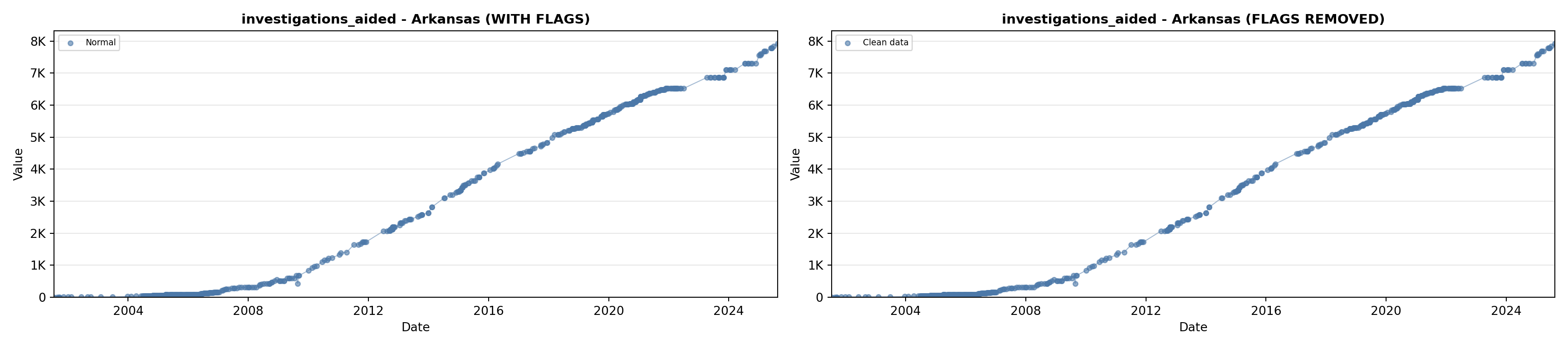
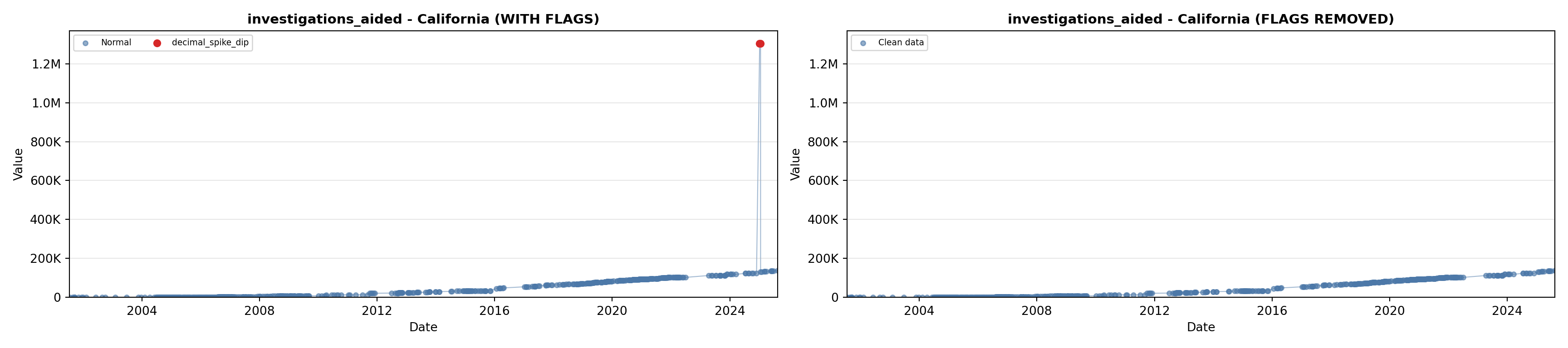
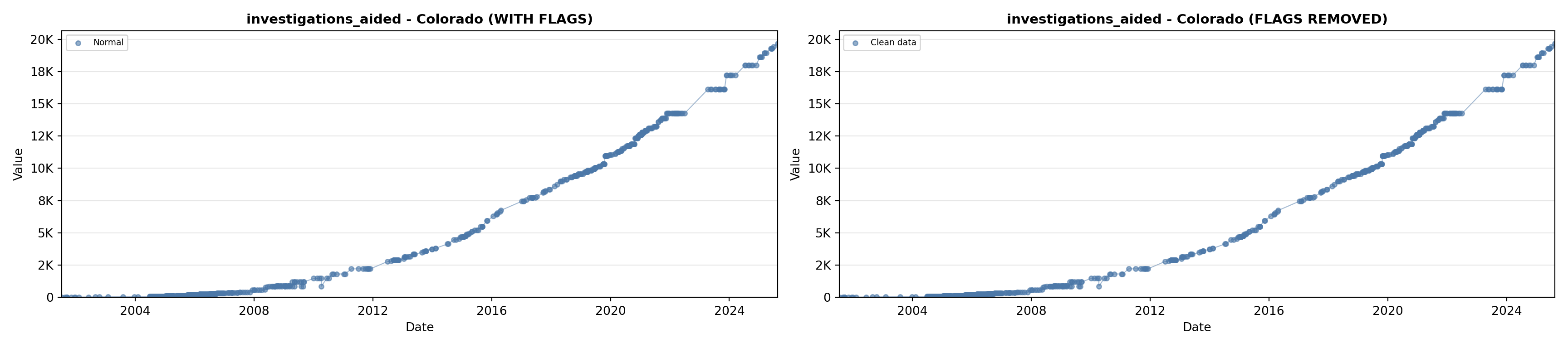
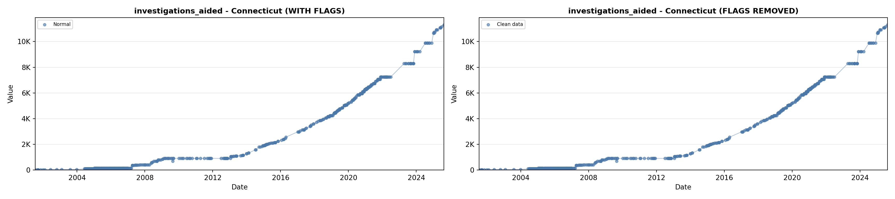
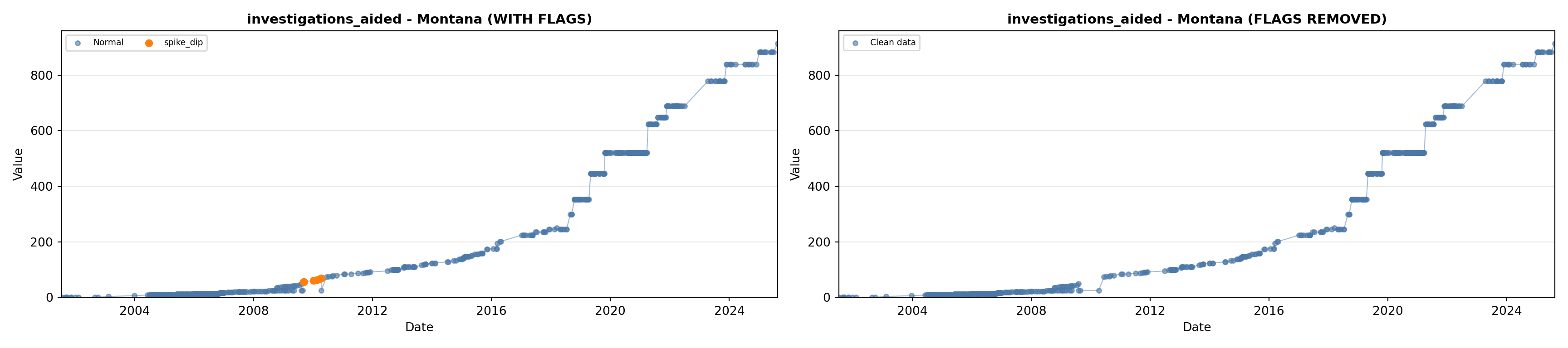
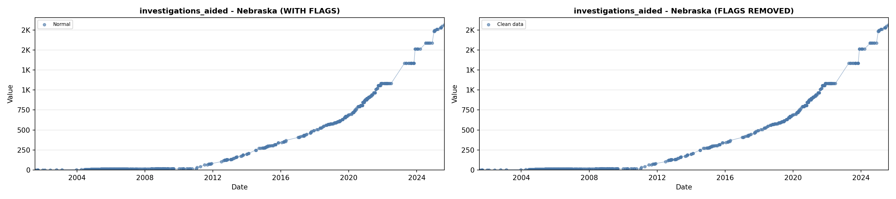
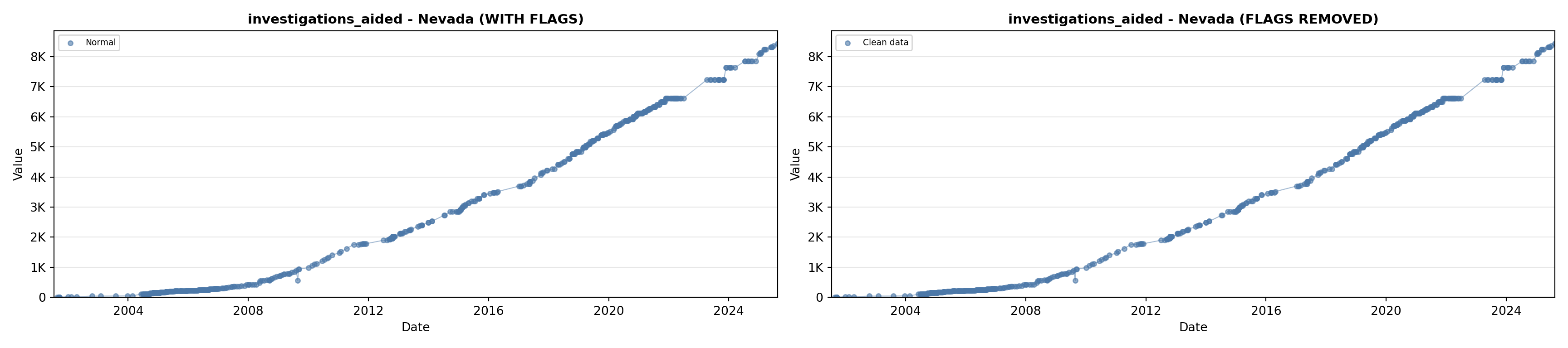
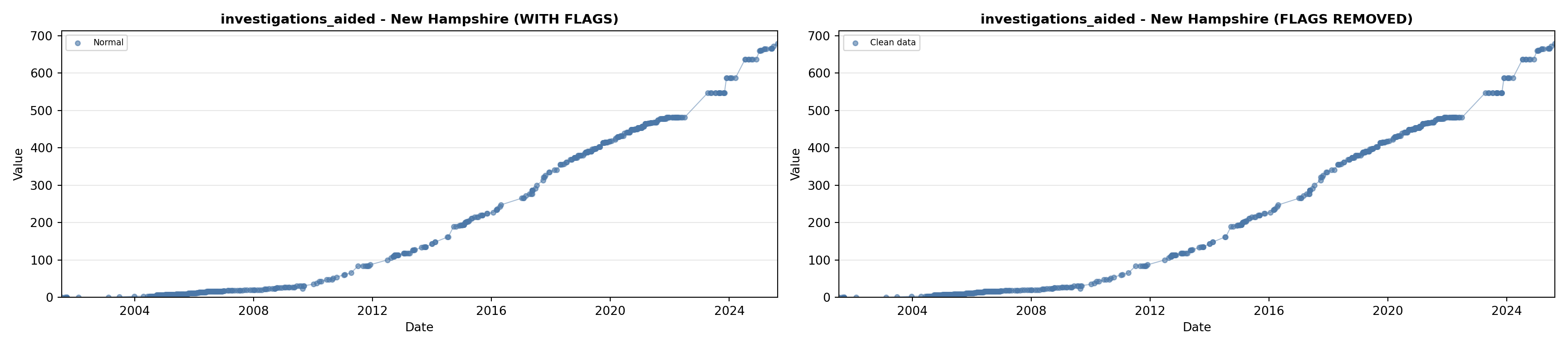
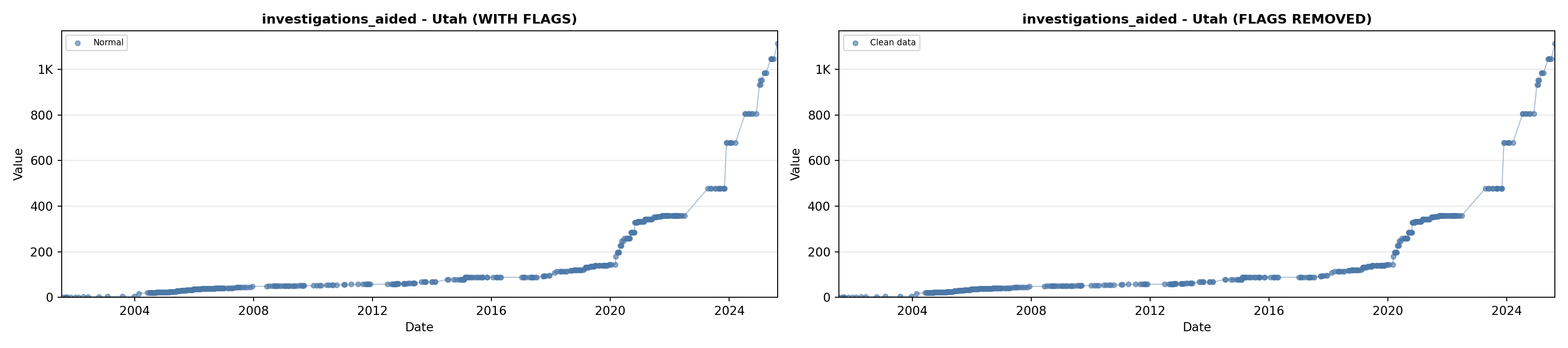
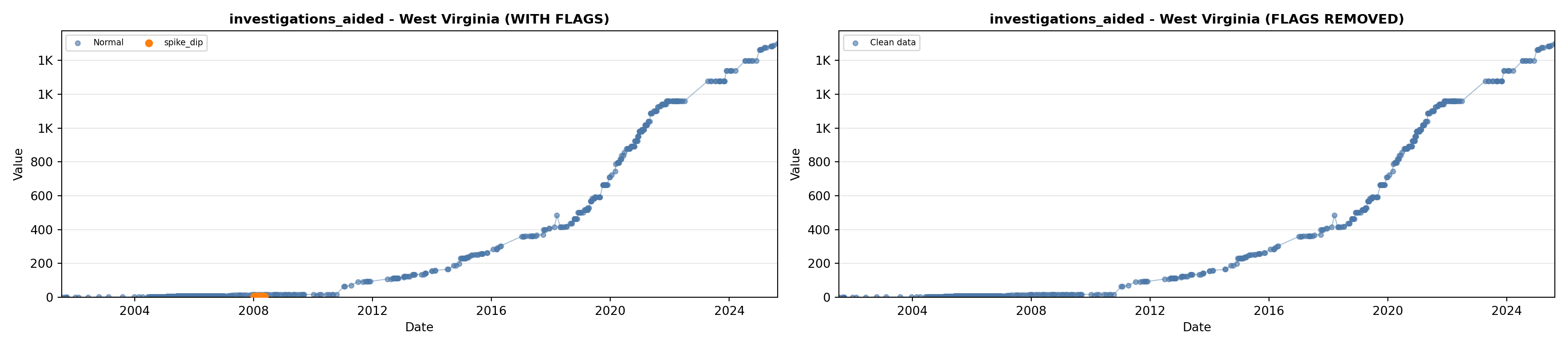
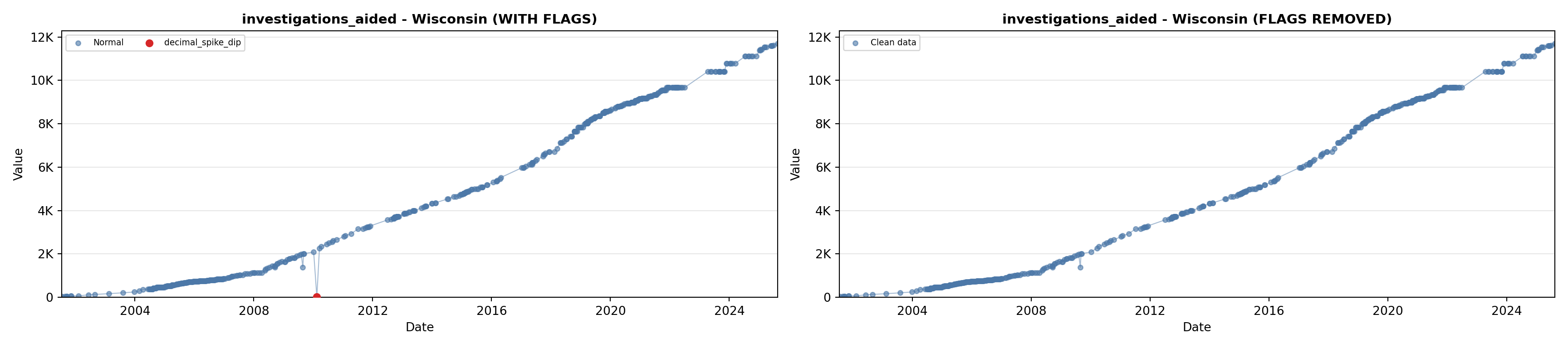
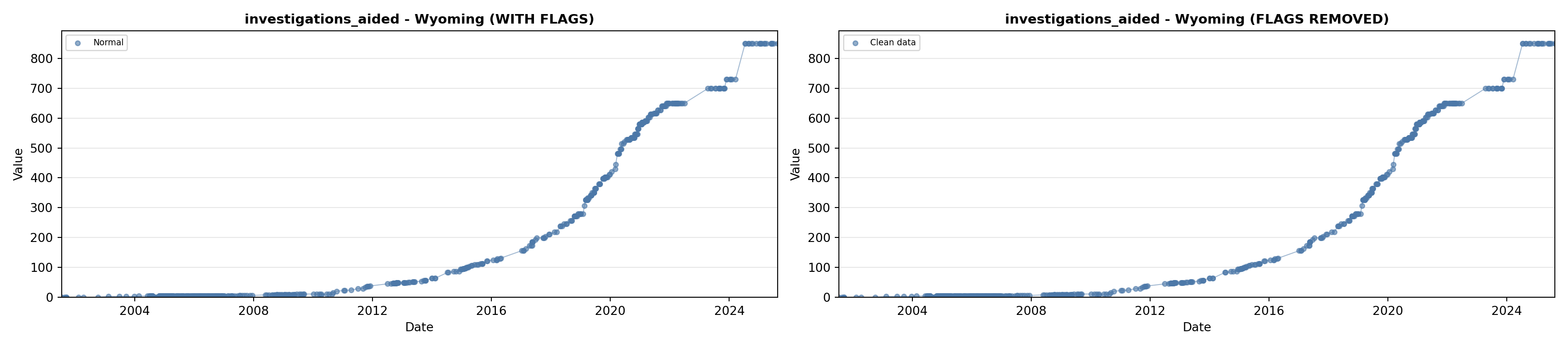
# 5. Investigations Aided (full width at bottom)
investigations_lit <- filter(literature_data, !is.na(investigations_aided))
p5 <- ggplot() +
geom_line(data = growth_data, aes(x = date, y = investigations_aided),
color = investigations_color, linewidth = 0.8) +
geom_point(data = growth_data, aes(x = date, y = investigations_aided),
color = investigations_color, size = 1.5) +
geom_point(data = investigations_lit, aes(x = asof_date, y = investigations_aided),
shape = 4, size = 2.5, stroke = 1, color = investigations_color) +
geom_label_repel(
data = filter(investigations_lit, year(asof_date) < 2021),
aes(x = asof_date, y = investigations_aided, label = short_label),
size = label_size, nudge_y = 80000,
box.padding = 0.3, point.padding = 0.3, min.segment.length = 0.3,
segment.color = "gray50", direction = "both", max.overlaps = Inf,
fill = "white", label.size = 0.2
) +
geom_label_repel(
data = filter(investigations_lit, year(asof_date) == 2021),
aes(x = asof_date, y = investigations_aided, label = short_label),
size = label_size, nudge_y = 10000, nudge_x = 400,
box.padding = 0.3, point.padding = 0.3, min.segment.length = 0.3,
segment.color = "gray50", max.overlaps = Inf,
fill = "white", label.size = 0.2
) +
geom_label_repel(
data = filter(investigations_lit, year(asof_date) > 2021),
aes(x = asof_date, y = investigations_aided, label = short_label),
size = label_size, nudge_y = 15000, nudge_x = -300, direction = "x",
box.padding = 0.3, point.padding = 0.3, min.segment.length = 0.3,
segment.color = "gray50", max.overlaps = Inf,
fill = "white", label.size = 0.2
) +
scale_x_date(date_breaks = "2 years", date_labels = "%Y", limits = extended_date_range) +
scale_y_continuous(labels = scale_axis, limits = c(0, max(investigations_lit$investigations_aided, na.rm = TRUE) * 1.15),
expand = expansion(mult = c(0, 0.05))) +
labs(title = "(E) Investigations Aided", x = "Year", y = "Count") +
theme_crossref
# Combine plots - 3 rows: top row 2 plots, middle row 2 plots, bottom row full width
fig7_verification <- (p1 + p2) / (p3 + p4) / p5 +
plot_layout(heights = c(1, 1, 1)) +
plot_annotation(
title = "Cross-Validation: Our Data vs. Published Literature",
subtitle = "X markers show published values from FBI brochures and peer-reviewed papers",
theme = theme(plot.title = element_text(face = "bold", size = 14))
)
fig7_verification