This document provides complete transparency regarding the data sources and methodology used to compile racial disparities in DNA collection across U.S. states. The original data was collected in Summer 2017, with most data points from 2013-2016.
Key Findings
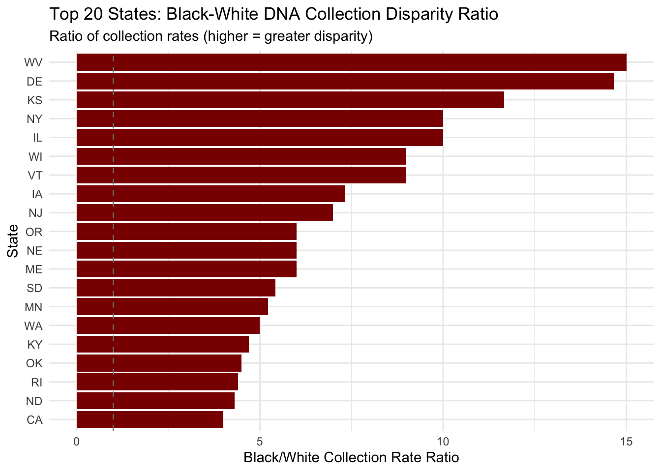
Consistent racial disparities: Black populations show the highest DNA collection rates relative to their population percentage in nearly all states
Data limitations: Many states lack comprehensive conviction data, requiring the use of prison admission proxies
Methodological challenges: Hispanic/Latino populations often uncounted or miscategorized in state data
Methodology Overview
Data Collection Period
Primary collection: Summer 2017
Data years used: Single year per state (2012-2016, varies by availability)
Census baseline: 2010 U.S. Census for demographic comparisons
General Challenges Encountered
Conviction Data Scarcity: Most states do not publicly disclose comprehensive felony conviction data
Prison Admission Proxy: Prison admissions used as substitute for conviction data in majority of states
Racial Classification Inconsistencies:
-   Many states only report "Black" and "White" categories

-   Hispanic/Latino often classified as ethnicity rather than race

-   "Other" category frequently used without specification
Arrest Data Gaps: Racial makeup of arrests often unavailable or incomplete
National Summary Table
Methodology: Parsing DNA Collection Data
The national summary data was extracted from a structured text file (MurphyTong_Racial_Breakdown.txt) containing three distinct data sections for each state:
DNA Collection Data: Percentage and absolute counts of DNA profiles collected by race (e.g., “46% B (18,253)”)
Population Demographics: Percentage of state population by race from 2010 Census
Processing Steps:
State Identification: The parser identifies state entries using standard two-letter abbreviations (AL, AK, AZ, etc.)
Section Segmentation: For each state, the text is divided into three sections based on the pattern of “% B” (Black percentage) occurrences
Data Extraction: Regular expressions extract both percentages and counts from the first section, and percentages only from the demographic and rate sections
Pattern Matching: The code uses regex patterns like ([0-9.]+)%\s*B\s*\(([0-9,]+)\) to capture both percentage (e.g., 46%) and count (e.g., 18,253) for DNA collection data
Race Categories: Data is extracted for five racial categories: Black (B), Hispanic (H), Asian (A), Native American (N), and White (W)
This automated parsing ensures reproducibility and allows for systematic extraction of data from the original Murphy & Tong study format.
Show summary code
# Function to parse DNA collection data from text fileparse_dna_data <-function(file_path) {# Read the entire file text_data <-readLines(file_path, warn =FALSE)# Remove empty lines text_data <- text_data[text_data !=""]# Initialize list to store parsed data parsed_data <-list()# State abbreviations (for reference) state_abbrevs <-c("AL", "AK", "AZ", "AR", "CA", "CO", "CT", "DE", "FL", "GA", "HI", "ID", "IL", "IN", "IA", "KS", "KY", "LA", "ME", "MD", "MA", "MI", "MN", "MS", "MO", "MT", "NE", "NV", "NH", "NJ", "NM", "NY", "NC", "ND", "OH", "OK", "OR", "PA", "RI", "SC", "SD", "TN", "TX", "UT", "VT", "VA", "WA", "WV", "WI", "WY", "DC")# Function to extract percentage and count from patterns like "46% B (18,253)" extract_race_data <-function(text, race_letter) { pattern <-paste0("([0-9.]+)%\\s*", race_letter, "\\s*\\(([0-9,]+)\\)") matches <-str_match(text, pattern)if (!is.na(matches[1])) { pct <-as.numeric(matches[2]) count <-as.numeric(gsub(",", "", matches[3]))return(list(pct = pct, count = count)) }return(list(pct =NA, count =NA)) }# Function to extract just percentage (for demographics and collection rates) extract_percentage <-function(text, race_letter) { pattern <-paste0("([0-9.]+)%\\s*", race_letter) matches <-str_match(text, pattern)if (!is.na(matches[1])) {return(as.numeric(matches[2])) }return(NA) }# Process each line i <-1while (i <=length(text_data)) { line <- text_data[i]# Check if line is a state abbreviationif (line %in% state_abbrevs) { state <- line# Initialize data structure for this state state_data <-list(State = state,Black_DNA_Pct =NA, Black_DNA_N =NA,Hispanic_DNA_Pct =NA, Hispanic_DNA_N =NA,Asian_DNA_Pct =NA, Asian_DNA_N =NA,Native_American_DNA_Pct =NA, Native_American_DNA_N =NA,White_DNA_Pct =NA, White_DNA_N =NA,Black_Pop_Pct =NA, Hispanic_Pop_Pct =NA, Asian_Pop_Pct =NA,Native_American_Pop_Pct =NA, White_Pop_Pct =NA,Black_Collection_Rate =NA, Hispanic_Collection_Rate =NA,Asian_Collection_Rate =NA, Native_American_Collection_Rate =NA,White_Collection_Rate =NA )# Collect all lines for this state until we hit the next state or end of file state_lines <-c() i <- i +1while (i <=length(text_data) &&!(text_data[i] %in% state_abbrevs)) { state_lines <-c(state_lines, text_data[i]) i <- i +1 }# Combine all lines for this state into one text block state_text <-paste(state_lines, collapse =" ")# Split into sections based on the pattern of % B occurrences# We need to identify the three sections: DNA Collection, Demographics, Collection Rates# Find all "% B" patterns to help identify sections b_patterns <-str_locate_all(state_text, "[0-9.]+%\\s*B")[[1]]if (nrow(b_patterns) >=1) {# First section: DNA Collection (has counts in parentheses) dna_section_start <-1 dna_section_end <-if(nrow(b_patterns) >=2) b_patterns[2,1] -1elsenchar(state_text) dna_section <-substr(state_text, dna_section_start, dna_section_end)# Extract DNA collection data (with counts) black_dna <-extract_race_data(dna_section, "B") hispanic_dna <-extract_race_data(dna_section, "H") asian_dna <-extract_race_data(dna_section, "A") native_dna <-extract_race_data(dna_section, "N") white_dna <-extract_race_data(dna_section, "W") state_data$Black_DNA_Pct <- black_dna$pct state_data$Black_DNA_N <- black_dna$count state_data$Hispanic_DNA_Pct <- hispanic_dna$pct state_data$Hispanic_DNA_N <- hispanic_dna$count state_data$Asian_DNA_Pct <- asian_dna$pct state_data$Asian_DNA_N <- asian_dna$count state_data$Native_American_DNA_Pct <- native_dna$pct state_data$Native_American_DNA_N <- native_dna$count state_data$White_DNA_Pct <- white_dna$pct state_data$White_DNA_N <- white_dna$count }if (nrow(b_patterns) >=2) {# Second section: Demographics (percentages only, no parentheses) demo_section_start <- b_patterns[2,1] demo_section_end <-if(nrow(b_patterns) >=3) b_patterns[3,1] -1elsenchar(state_text) demo_section <-substr(state_text, demo_section_start, demo_section_end)# Extract demographic percentages state_data$Black_Pop_Pct <-extract_percentage(demo_section, "B") state_data$Hispanic_Pop_Pct <-extract_percentage(demo_section, "H") state_data$Asian_Pop_Pct <-extract_percentage(demo_section, "A") state_data$Native_American_Pop_Pct <-extract_percentage(demo_section, "N") state_data$White_Pop_Pct <-extract_percentage(demo_section, "W") }if (nrow(b_patterns) >=3) {# Third section: Collection Rates (percentages only, no parentheses) rate_section_start <- b_patterns[3,1] rate_section <-substr(state_text, rate_section_start, nchar(state_text))# Extract collection rate percentages state_data$Black_Collection_Rate <-extract_percentage(rate_section, "B") state_data$Hispanic_Collection_Rate <-extract_percentage(rate_section, "H") state_data$Asian_Collection_Rate <-extract_percentage(rate_section, "A") state_data$Native_American_Collection_Rate <-extract_percentage(rate_section, "N") state_data$White_Collection_Rate <-extract_percentage(rate_section, "W") }# Add to parsed data parsed_data[[length(parsed_data) +1]] <- state_data# Don't increment i here since we already did it in the while loop i <- i -1 } i <- i +1 }# Convert to data frame df <-do.call(rbind, lapply(parsed_data, data.frame))return(df)}racial_data_path <-file.path(here("data", "annual_dna_collection", "intermediate", "MurphyTong_Racial_Breakdown.txt"))summary_data <-parse_dna_data(racial_data_path)# Display interactive tabledatatable(summary_data, options =list(pageLength =10, scrollX =TRUE),caption ="Complete state-by-state breakdown of DNA collection by race")
Table 1: Racial Breakdown of Annual DNA Collection for Each State
Figure 1: DNA Collection Rates by Race Relative to Population Percentage
State-by-State Detailed Methodology
Methodology: Parsing State Methodology Paragraphs
The detailed methodology for each state was extracted from a separate text file (MurphyTong_States_Paragraphs.txt) containing narrative descriptions of data collection approaches for all 50 states. This section explains how we systematically parsed this unstructured text into a structured dataset.
Processing Steps:
State Detection: The parser identifies state entries by searching for the 50 U.S. state names as they appear in the text
Section Extraction: For each state, the parser captures all text from the state name until the next state name appears
Component Parsing: Within each state’s section, the code extracts four key components:
Legal Framework: The statutory basis for DNA collection in that state
Collection Triggers: Specific offenses or events that trigger DNA collection
Data Sources: Types of data used (e.g., conviction records, prison admissions, arrest data)
Source URLs: Web links to the original data sources
Data Limitations: Known gaps, proxies, or methodological caveats
Structured Data Creation: Each data source line is parsed into a type-note pair (e.g., “Prison admissions: Used as proxy for conviction data”)
Categorization: The parser automatically categorizes:
Collection trigger types: Comprehensive, selective, felony-only, etc.
Data limitation types: Missing conviction data, ethnicity issues, limited racial categories, etc.
Data source types: Conviction data, arrest data, prison data, sex crime data, etc.
This systematic extraction allows for consistent comparison across states and identification of common patterns in data collection methodologies and limitations.
Show paragraph extraction code
# Pre-define all 50 U.S. statesus_states <-c("Alabama", "Alaska", "Arizona", "Arkansas", "California", "Colorado", "Connecticut", "Delaware", "Florida", "Georgia", "Hawaii", "Idaho", "Illinois", "Indiana", "Iowa", "Kansas", "Kentucky", "Louisiana", "Maine", "Maryland", "Massachusetts", "Michigan", "Minnesota", "Mississippi", "Missouri", "Montana", "Nebraska", "Nevada", "New Hampshire", "New Jersey", "New Mexico", "New York", "North Carolina", "North Dakota", "Ohio", "Oklahoma", "Oregon", "Pennsylvania", "Rhode Island", "South Carolina", "South Dakota", "Tennessee", "Texas", "Utah", "Vermont", "Virginia", "Washington", "West Virginia", "Wisconsin", "Wyoming")# Read the text filedata_file <-file.path(here("data", "annual_dna_collection", "intermediate", "MurphyTong_States_Paragraphs.txt"))text_content <-readLines(data_file, warn =FALSE)# Combine all lines into a single stringfull_text <-paste(text_content, collapse ="\n")# Create a pattern to match state namesstate_pattern <-paste0("(?m)^[[:space:]]*(", paste(us_states, collapse ="|"), ")\\b")state_matches <-str_locate_all(full_text, state_pattern)[[1]]# Extract state sectionsstate_sections <-list()state_names <-character()if (nrow(state_matches) >0) {for (i in1:nrow(state_matches)) { start_pos <- state_matches[i, "start"]if (i <nrow(state_matches)) { end_pos <- state_matches[i +1, "start"] -1 } else { end_pos <-nchar(full_text) } state_name <-substr(full_text, start_pos, state_matches[i, "end"]) state_content <-substr(full_text, start_pos, end_pos) state_names <-c(state_names, state_name) state_sections <-c(state_sections, state_content) }}# Function to extract information from each state sectionparse_state_section <-function(section, state_name) {if (is.na(state_name)) return(NULL)# Extract legal framework legal_framework <-str_extract(section, "Legal Framework:[^\n]+") %>% {ifelse(is.na(.), NA, str_remove(., "Legal Framework:") %>%str_trim())}# Extract collection triggers collection_triggers <-str_extract(section, "Collection Triggers:[^\n]+") %>% {ifelse(is.na(.), NA, str_remove(., "Collection Triggers:") %>%str_trim())}# Extract data sources - capture everything until Source URLs or Data Limitations data_sources_text <-str_extract(section, "Data Sources:[\\s\\S]*?(?=Source URLs:|Data Limitations:|$)") data_source_df <-tibble(data_source_type =NA_character_, data_source_note =NA_character_)if (!is.na(data_sources_text)) { data_sources_text <-str_remove(data_sources_text, "Data Sources:") %>%str_trim()# Split by newlines and clean up data_source_lines <-str_split(data_sources_text, "\\n")[[1]] %>%str_trim() %>%discard(~ .x ==""|str_detect(.x, "^Source URLs:|^Data Limitations:"))if (length(data_source_lines) >0) { data_source_df <-map_df(data_source_lines, function(line) {if (str_detect(line, ":")) {tibble(data_source_type =str_extract(line, "^[^:]+") %>%str_trim(),data_source_note =str_remove(line, "^[^:]+:") %>%str_trim() ) } else {tibble(data_source_type = line,data_source_note =NA_character_ ) } }) } }# Extract source URLs source_urls_text <-str_extract(section, "Source URLs:[\\s\\S]*?(?=Data Limitations:|$)") source_urls <-character(0)if (!is.na(source_urls_text)) { source_urls_text <-str_remove(source_urls_text, "Source URLs:") %>%str_trim() source_url_lines <-str_split(source_urls_text, "\\n")[[1]] %>%str_trim() %>%discard(~ .x ==""|str_detect(.x, "^Data Limitations:"))if (length(source_url_lines) >0) { source_urls <- source_url_lines } }# Extract data limitations - capture everything until next state or end data_limitations_text <-str_extract(section, "Data Limitations:[\\s\\S]*?(?=\\b(A|Ala|Alas|Ari|Arka|Cali|Colo|Conn|Del|Flo|Geo|Haw|Ida|Ill|Ind|Iow|Kan|Ken|Lou|Mai|Mar|Mas|Mic|Min|Mis|Mon|Neb|Nev|New|Nor|Ohi|Okl|Ore|Pen|Rho|Sou|Ten|Tex|Uta|Ver|Vir|Was|Wis|Wyo)\\b|$)") data_limitations <-NA_character_if (!is.na(data_limitations_text)) { data_limitations_text <-str_remove(data_limitations_text, "Data Limitations:") %>%str_trim() data_limitations_lines <-str_split(data_limitations_text, "\\n")[[1]] %>%str_trim() %>%discard(~ .x ==""|str_detect(.x, "^\\b(A|Ala|Alas|Ari|Arka|Cali|Colo|Conn|Del|Flo|Geo|Haw|Ida|Ill|Ind|Iow|Kan|Ken|Lou|Mai|Mar|Mas|Mic|Min|Mis|Mon|Neb|Nev|New|Nor|Ohi|Okl|Ore|Pen|Rho|Sou|Ten|Tex|Uta|Ver|Vir|Was|Wis|Wyo)\\b"))if (length(data_limitations_lines) >0) { data_limitations <-paste(data_limitations_lines, collapse ="; ") } }# If no data sources were found, create at least one row for the stateif (nrow(data_source_df) ==0) { data_source_df <-tibble(data_source_type =NA_character_, data_source_note =NA_character_) }# Create result dataframe result_df <- data_source_df %>%mutate(state = state_name,legal_framework = legal_framework,collection_triggers = collection_triggers,source_url =ifelse(length(source_urls) >0, paste(source_urls, collapse ="; "), NA_character_),data_limitations = data_limitations,.before =everything() )return(result_df)}# Parse all state sectionsstate_data_list <-lapply(seq_along(state_sections), function(i) {parse_state_section(state_sections[[i]], state_names[i])})# Combine all results into one dataframestate_data <-bind_rows(state_data_list)# Clean up the data - remove rows where all data columns are NAfinal_df <- state_data %>%mutate(across(where(is.character), ~ifelse(.x ==""|is.na(.x), NA, .x))) %>%filter(!(is.na(data_source_type) &is.na(source_url) &is.na(data_limitations)))# Fill in the missing legal_framework and other methodology for each statefinal_df_clean <- final_df %>%group_by(state) %>%fill(legal_framework, collection_triggers, .direction ="downup") %>%ungroup()# Now let's fill source_url and data_limitations across all rows for each statefinal_df_clean <- final_df_clean %>%group_by(state) %>%mutate(source_url =ifelse(all(is.na(source_url)), NA, paste(na.omit(unique(source_url)), collapse ="; ")),data_limitations =ifelse(all(is.na(data_limitations)), NA,paste(na.omit(unique(data_limitations)), collapse ="; ")) ) %>%ungroup()# Create categorization columns for easier analysisfinal_df_clean <- final_df_clean %>%mutate(# Categorize collection triggerscollection_trigger_category =case_when(str_detect(collection_triggers, "(?i)all felony.*convictions.*arrests.*all felonies") ~"Comprehensive: All felonies + broad arrests",str_detect(collection_triggers, "(?i)all felony.*convictions.*arrests.*certain|specific") ~"Selective: All felonies + specific arrests",str_detect(collection_triggers, "(?i)all felony.*convictions.*arrests") ~"Broad: All felonies + various arrests",str_detect(collection_triggers, "(?i)all felony.*convictions") ~"Felony convictions only",str_detect(collection_triggers, "(?i)felony.*misdemeanor.*convictions") ~"Mixed: Felony + misdemeanor convictions",TRUE~"Other/Unspecified" ),# Categorize data limitationsdata_limitation_category =case_when(is.na(data_limitations) ~"No limitations noted",str_detect(data_limitations, "(?i)no direct.*conviction data") ~"Missing conviction data",str_detect(data_limitations, "(?i)prison admissions.*proxy") ~"Prison data as proxy",str_detect(data_limitations, "(?i)hispanic|ethnicity") ~"Ethnicity categorization issues",str_detect(data_limitations, "(?i)racial.*limited|black.*white.*only") ~"Limited racial categories",str_detect(data_limitations, "(?i)no.*data.*available|unavailable") ~"Various data unavailable",TRUE~"Other limitations" ),# Categorize data source typesdata_source_category =case_when(str_detect(data_source_type, "(?i)conviction") ~"Conviction Data",str_detect(data_source_type, "(?i)arrest") ~"Arrest Data",str_detect(data_source_type, "(?i)sex|sexual") ~"Sex Crime Data",str_detect(data_source_type, "(?i)prison|admission|correction") ~"Prison/Incarceration Data",TRUE~"Other Data Source" ) )# Create a summary table for quick overview - ONE ROW PER STATEmethodology_summary <- final_df_clean %>%distinct(state, legal_framework, collection_triggers, collection_trigger_category, data_limitations, data_limitation_category, source_url) %>%arrange(state) %>%mutate(state =str_trim(state))# Create interactive tabledatatable_methodology <-datatable( methodology_summary,extensions =c('Buttons', 'ColReorder', 'Scroller'),options =list(dom ='Bfrtip',buttons =c('copy', 'csv', 'excel', 'colvis'),scrollX =TRUE,scrollY ="600px",scroller =TRUE,pageLength =10,columnDefs =list(list(className ='dt-left', targets =0:(ncol(methodology_summary)-1)),list(width ='200px', targets =c(1, 2, 3)) ),autoWidth =TRUE ),rownames =FALSE,filter ='top',class ='cell-border stripe hover') %>%formatStyle(columns =names(methodology_summary),fontSize ='12px',lineHeight ='90%' )# Show the tabledatatable_methodology
Combining Information into Master Dataset
The final dataset combines quantitative DNA collection metrics with qualitative methodology to create a comprehensive one-row-per-state resource. This integration allows researchers to understand both the magnitude of DNA collection and the quality/limitations of the underlying data sources.
Integration Process:
Primary Dataset: The summary_data table contains all quantitative metrics:
DNA collection counts and percentages by race
State population demographics by race
Collection rates per 100,000 population by race
Study Methodology Addition: The methodology_summary table provides contextual information:
Legal framework for DNA collection
Specific collection triggers
Data source types and limitations
Source URLs for verification
Joining Strategy:
States are matched using full state names
A crosswalk table converts two-letter abbreviations to full names
Left join ensures all states from the summary data are retained
Column Selection: The final dataset includes:
State identifier: Full state name
Collection metrics: All DNA collection counts, percentages, and rates by race
Methodology context: Legal framework, collection triggers, data limitations
Quality flags: Categorized data limitation types for filtering/analysis
Output Format: One row per state with 30+ columns covering demographics, collection rates, and methodology
This unified structure enables analyses that account for data quality differences across states when interpreting racial disparities in DNA collection.
# Create output directory structureintermediate_dir <-here("data", "annual_dna_collection", "intermediate")dir.create(intermediate_dir, recursive =TRUE, showWarnings =FALSE)final_dir <-here("data", "annual_dna_collection", "final")dir.create(final_dir, recursive =TRUE, showWarnings =FALSE)# Export final combined datasetoutput_path <-file.path(final_dir, "Annual_DNA_Collection.csv")write_csv(annual_dna_combined, output_path)cat(paste("✓ Exported Annual DNA Collection dataset to:", output_path, "\n"))# Also export the methodology summary separately for referencemethodology_output_path <-file.path(intermediate_dir, "State_Methodology.csv")write_csv(methodology_summary, methodology_output_path)cat(paste("✓ Exported study methodology summary to:", methodology_output_path, "\n"))cat("Use analysis/version_freeze.qmd to create processed data releases when needed.\n")
✓ Exported Annual DNA Collection dataset to: /Users/tlasisi/GitHub/PODFRIDGE-Databases/data/annual_dna_collection/final/Annual_DNA_Collection.csv
✓ Exported study methodology summary to: /Users/tlasisi/GitHub/PODFRIDGE-Databases/data/annual_dna_collection/intermediate/State_Methodology.csv
Use analysis/version_freeze.qmd to create processed data releases when needed.
Summary and Key Findings
Dataset Completeness
Show completeness analysis
# Analyze data completeness by categorycompleteness_summary <- annual_dna_combined %>%summarise(States_with_Black_Data =sum(!is.na(Black_Collection_Rate)),States_with_Hispanic_Data =sum(!is.na(Hispanic_Collection_Rate)),States_with_Asian_Data =sum(!is.na(Asian_Collection_Rate)),States_with_Native_American_Data =sum(!is.na(Native_American_Collection_Rate)),States_with_White_Data =sum(!is.na(White_Collection_Rate)),States_with_Legal_Framework =sum(!is.na(legal_framework)) )kable(t(completeness_summary), col.names ="Count", caption ="Data Completeness Across States") %>%kable_styling(bootstrap_options =c("striped", "hover"))