Simulate the number of relatives under different fertility and sibling models

1 Simulate the number of relatives

We simulate the number of relatives for each individual using fertility and sibling distributions.

The simulation uses a fixed two-parent pedigree anchor to connect focal individuals to parental and grandparental generations. The reported counts are the kin classes generated from fertility or size-biased sibling distributions: children, siblings, aunts/uncles, nieces/nephews, and first cousins.

For an interactive version of the same model, see the Kincounts simulator.

1.1 Simulate the relative counts for the focal individual

This code defines the kin-count simulator under ZINB, Poisson, and fixed-mean fertility assumptions. The two-parent anchor is used internally for aunts/uncles and cousins, but parents and grandparents are not reported as modeled outcomes.

# The fertility distribution modeled as a zero-inflated negative binomial distribution.
simulate_relatives_zinb <- function(mus, sizes, pis,
                                    n_sim = 10000,
                                    max_kids = 12) {
  draw_fert <- function(n, mu, size, pi) {
    ifelse(runif(n) < pi, 0L,
           as.integer(pmin(rnbinom(n, size, mu = mu), max_kids)))
  }
  
  draw_sibs <- function(n, mu, size) {
    as.integer(pmin(rnbinom(n, size + 1, mu = mu * (size + 1) / size), max_kids - 1))
  }
  sum_fert <- function(counts, gen) {
    purrr::map_int(counts, function(n) {
      if (n == 0L) 0L else as.integer(sum(draw_fert(n, mu = mus[gen], size = sizes[gen], pi = pis[gen])))
    })
  }
  sum_sibs <- function(counts, gen) {
    purrr::map_int(counts, function(n) {
      if (n == 0L) 0L else as.integer(sum(draw_sibs(n, mu = mus[gen], size = sizes[gen])))
    })
  }
  # 1. Parents are a fixed pedigree anchor used to generate aunts and uncles.
  parents <- rep(2L, n_sim)

  # 2. Siblings for the focal individual
  siblings <- draw_sibs(n = n_sim, mu = mus[2], size = sizes[2])
  
  # 3. Children of the focal individual
  children <- draw_fert(n = n_sim, mu = mus[1], size = sizes[1], pi = pis[1])

  # 4. Aunts & uncles (no subtraction needed)
  aunts_uncles <- sum_sibs(parents, gen = 3)

  # 5. Nieces & nephews: for each sibling, simulate their fertility and sum
  nieces_nephews <- sum_fert(siblings, gen = 1)

  # 6. Cousins: for each aunt/uncle, simulate their fertility and sum
  cousins <- sum_fert(aunts_uncles, gen = 2)

  tibble::tibble(
    Siblings    = siblings,
    Children    = children,
    AuntUncles = aunts_uncles,
    NieceNephews = nieces_nephews,
    Cousins = cousins
  )
}

# The fertility distribution modeled as a Poisson distribution.
simulate_relatives_poisson <- function(mus, 
                                       n_sim = 10000,
                                       max_kids = 12) {
  draw_fert <- function(n, mu) {
    as.integer(pmin(rpois(n, lambda = mu), max_kids))
  }
  
  draw_sibs <- function(n, mu, size) {
    as.integer(pmin(rpois(n, lambda = mu), max_kids - 1))
  }
  sum_fert <- function(counts, gen) {
    purrr::map_int(counts, function(n) {
      if (n == 0L) 0L else as.integer(sum(draw_fert(n, mu = mus[gen])))
    })
  }
  sum_sibs <- function(counts, gen) {
    purrr::map_int(counts, function(n) {
      if (n == 0L) 0L else as.integer(sum(draw_sibs(n, mu = mus[gen])))
    })
  }
  # 1. Parents are a fixed pedigree anchor used to generate aunts and uncles.
  parents <- rep(2L, n_sim)

  # 2. Siblings for the focal individual
  siblings <- draw_sibs(n = n_sim, mu = mus[2])
  
  # 3. Children of the focal individual
  children <- draw_fert(n = n_sim, mu = mus[1])

  # 4. Aunts & uncles (no subtraction needed)
  aunts_uncles <- sum_sibs(parents, gen = 3)

  # 5. Nieces & nephews: for each sibling, simulate their fertility and sum
  nieces_nephews <- sum_fert(siblings, gen = 1)

  # 6. Cousins: for each aunt/uncle, simulate their fertility and sum
  cousins <- sum_fert(aunts_uncles, gen = 2)

  tibble::tibble(
    Siblings    = siblings,
    Children    = children,
    AuntUncles = aunts_uncles,
    NieceNephews = nieces_nephews,
    Cousins = cousins
  )
}

# The fertility distribution fixed at the mean size.
simulate_relatives_fixed <- function(ferts, sibs) {
  # 1. Parents are a fixed pedigree anchor used to generate aunts and uncles.
  parents <- 2

  # 2. Siblings for the focal individual
  siblings <- sibs[2]
  
  # 3. Children of the focal individual
  children <- ferts[1]

  # 4. Aunts & uncles (no subtraction needed)
  aunts_uncles <- parents * sibs[3]

  # 5. Nieces & nephews: for each sibling, simulate their fertility and sum
  nieces_nephews <- siblings * ferts[1]

  # 6. Cousins: for each aunt/uncle, simulate their fertility and sum
  cousins <- aunts_uncles * ferts[2]

  tibble::tibble(
    Siblings    = siblings,
    Children    = children,
    AuntUncles = aunts_uncles,
    NieceNephews = nieces_nephews,
    Cousins = cousins
  )
}

1.2 Fertility and sibling parameters based on the IPUMS data

The notebook reads fitted parameters and empirical sibling moments from the current analysis outputs, keeping these simulations synchronized with the fertility-model notebook.

# Read the fitted parameters and empirical summaries written by fert_model.qmd
# instead of hard-coding them, so this notebook stays in sync with the data.
fert_params <- read_csv(file.path(output_path, "fertility_parameters.csv"), show_col_types = FALSE)
fert_estimation <- read_csv(file.path(output_path, "fertility_estimation.csv"), show_col_types = FALSE)

zinb_params <- fert_params %>% filter(Model == "ZINB")
pois_params <- fert_params %>% filter(Model == "Poisson")
sib_estimation <- fert_estimation %>% filter(distribution == "sibling")

all_census_years <- sort(unique(zinb_params$Year))

# Generations used in the kin-count simulation below, in order:
# focal individual, parent, grandparent.
gen_years <- c(1990, 1970, 1950)

mus_zinb <- zinb_params$mu[match(gen_years, zinb_params$Year)]
sizes_zinb <- zinb_params$size[match(gen_years, zinb_params$Year)]
pis_zinb <- zinb_params$pi0[match(gen_years, zinb_params$Year)]
mus_poisson <- pois_params$mu[match(gen_years, pois_params$Year)]
mean_ferts <- mus_poisson
mean_sibs <- sib_estimation$mean_data[match(gen_years, sib_estimation$Year)]

n_sim <- 100000

1.3 Fertility and sibling model-fit PMFs

These plots mirror the simulator view: empirical bars, with ZINB and Poisson model overlays. We show every census year with fitted data here; the kin-count simulation below then selects three years as a focal-parent-grandparent generation mapping.

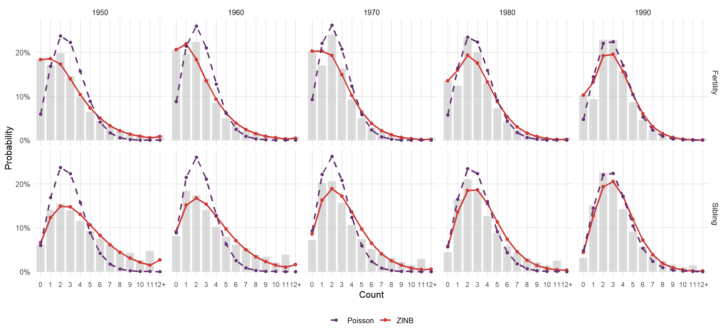
max_input_count <- 12L

zinb_pmf <- function(k, mu, size, pi0) {
  ifelse(
    k == 0L,
    pi0 + (1 - pi0) * dnbinom(k, size = size, mu = mu),
    (1 - pi0) * dnbinom(k, size = size, mu = mu)
  )
}

tail_pmf <- function(values) {
  pmax(0, 1 - sum(values))
}

model_pmf_for_year <- function(year) {
  z <- zinb_params %>% filter(Year == year)
  p <- pois_params %>% filter(Year == year)
  k <- 0:(max_input_count - 1L)

  fert_zinb <- zinb_pmf(k, mu = z$mu, size = z$size, pi0 = z$pi0)
  fert_pois <- dpois(k, lambda = p$mu)
  sib_zinb <- dnbinom(k, size = z$size + 1, mu = z$mu * (z$size + 1) / z$size)
  sib_pois <- dpois(k, lambda = p$mu)

  bind_rows(
    tibble(Year = year, Distribution = "Fertility", Count = c(k, max_input_count),
           poissonFit = c(fert_pois, tail_pmf(fert_pois)),
           zinbFit = c(fert_zinb, tail_pmf(fert_zinb))),
    tibble(Year = year, Distribution = "Sibling", Count = c(k, max_input_count),
           poissonFit = c(sib_pois, tail_pmf(sib_pois)),
           zinbFit = c(sib_zinb, tail_pmf(sib_zinb)))
  )
}

emp_fert_pmf <- read_csv(
  file.path(processed_path, "ipums_fertility_pmf_by_cohort.csv"),
  show_col_types = FALSE
) %>%
  filter(Year %in% all_census_years) %>%
  group_by(Year, cohort, Count = pmin(children, max_input_count)) %>%
  summarise(empirical = sum(probability), .groups = "drop") %>%
  mutate(Distribution = "Fertility")

emp_sib_pmf <- emp_fert_pmf %>%
  filter(Distribution == "Fertility") %>%
  group_by(Year, cohort) %>%
  group_modify(~ {
    probs <- numeric(max_input_count + 1L)
    probs[.x$Count + 1L] <- .x$empirical
    fert_mean <- fert_estimation$mean_data[
      fert_estimation$distribution == "fertility" &
        fert_estimation$Year == .y$Year
    ]
    known <- (1:max_input_count) * probs[2:(max_input_count + 1L)] / fert_mean
    tibble(
      Count = 0:max_input_count,
      empirical = c(known, pmax(0, 1 - sum(known))),
      Distribution = "Sibling"
    )
  }) %>%
  ungroup()

input_model_pmf <- bind_rows(lapply(all_census_years, model_pmf_for_year))

input_pmf <- bind_rows(emp_fert_pmf, emp_sib_pmf) %>%
  left_join(input_model_pmf, by = c("Year", "Distribution", "Count")) %>%
  mutate(
    CountLabel = factor(
      if_else(Count == max_input_count, paste0(max_input_count, "+"), as.character(Count)),
      levels = c(as.character(0:(max_input_count - 1L)), paste0(max_input_count, "+"))
    ),
    Year = factor(Year, levels = all_census_years),
    Distribution = factor(Distribution, levels = c("Fertility", "Sibling"))
  )

ggplot(input_pmf, aes(x = CountLabel)) +
  geom_col(aes(y = empirical), fill = empirical_fill, alpha = 0.65, width = 0.82) +
  geom_line(aes(y = zinbFit, group = 1, color = "ZINB"), linewidth = 1) +
  geom_point(aes(y = zinbFit, color = "ZINB"), size = 1.8) +
  geom_line(aes(y = poissonFit, group = 1, color = "Poisson"), linewidth = 0.9, linetype = "dashed") +
  geom_point(aes(y = poissonFit, color = "Poisson"), size = 1.6) +
  facet_grid(Distribution ~ Year) +
  scale_color_manual(values = model_fit_palette, name = NULL) +
  scale_y_continuous(labels = function(x) paste0(round(100 * x), "%")) +
  labs(x = "Count", y = "Probability") +
  theme_minimal(base_size = 12) +
  theme(
    legend.position = "bottom",
    panel.grid.minor = element_blank(),
    axis.text.x = element_text(size = 9)
  )

ggsave(file = file.path(output_path, "fertility_sibling_model_fit_pmf.pdf"), width = 13, height = 6)

1.4 Simulate relative counts for each fertility and sibling model

We run the relationship calculations under fixed-mean, Poisson, and ZINB assumptions. The illustrative generation mapping is focal = 1990, parent = 1970, and grandparent = 1950, corresponding to roughly 20-year generational spacing.

relative_counts <- list(
  # Fixed-mean baseline: replace each draw with the empirical mean.
  fixed = simulate_relatives_fixed(
    ferts = mean_ferts,
    sibs = mean_sibs
  ),
  # Poisson model: simulate fertility with one mean parameter per generation.
  poisson = simulate_relatives_poisson(
    mus = mus_poisson,
    n_sim = n_sim
  ),
  # ZINB model: simulate fertility with fitted mean, dispersion, and zero inflation.
  zinb = simulate_relatives_zinb(
    mus = mus_zinb,
    sizes = sizes_zinb,
    pis = pis_zinb,
    n_sim = n_sim
  )
)

1.5 Summarize mean and variance of relative counts

The summary table reports only modeled or fertility-derived kin counts; fixed parents and grandparents are treated as pedigree assumptions rather than outcomes.

relative_model_names <- names(relative_counts)

relative_summary <- Map(function(dat, model_name) {
  tibble(
    Relative = names(dat),
    mean = as.numeric(colMeans(dat)),
    variance = if (model_name == "fixed") {
      rep(0, ncol(dat))
    } else {
      as.numeric(sapply(dat, var))
    },
    model = model_name
  )
}, relative_counts, relative_model_names) %>%
  bind_rows()

relative_summary_table <- relative_summary %>%
  pivot_wider(
    names_from = model,
    values_from = c(mean, variance),
    names_glue = "{.value}_{model}"
  ) %>%
  dplyr::select(
    Relative,
    mean_fixed,
    mean_poisson,
    mean_zinb,
    variance_fixed,
    variance_poisson,
    variance_zinb
  )

write.csv(relative_summary_table, file.path(output_path, "relative_summary_table.csv"), row.names = FALSE)

kable(
  relative_summary_table,
  digits = 3,
  caption = "Mean and variance of relative counts by fertility and sibling model."
)

Mean and variance of relative counts by fertility and sibling model.

Relative	mean_fixed	mean_poisson	mean_zinb	variance_fixed	variance_poisson	variance_zinb
Siblings	3.344	2.371	3.243	0	2.387	5.382
Children	3.047	3.048	3.042	0	3.053	4.073
AuntUncles	8.383	5.635	8.246	0	5.579	16.213
NieceNephews	10.187	7.231	9.883	0	29.377	63.173
Cousins	19.927	13.382	19.569	0	44.827	127.679

1.6 Visualize relative count distributions as boxplots

The boxplots summarize the simulated count distributions and make the model-level shifts in medians and tails easy to compare.

relative_labels <- c(
  Siblings = "Siblings",
  Children = "Children",
  AuntUncles = "Aunts and uncles",
  NieceNephews = "Nieces and nephews",
  Cousins = "First cousins"
)

relative_levels <- c(
  "Siblings", "Children", "Aunts and uncles",
  "Nieces and nephews", "First cousins"
)

relative_distribution <- bind_rows(
  relative_counts$poisson %>% mutate(Model = "Poisson"),
  relative_counts$zinb %>% mutate(Model = "ZINB")
) %>%
  pivot_longer(
    cols = -Model,
    names_to = "Relative",
    values_to = "Count"
  ) %>%
  mutate(
    Relative = recode(Relative, !!!relative_labels),
    Relative = factor(Relative, levels = relative_levels)
  )

ggplot(relative_distribution, aes(x = Model, y = Count, fill = Model)) +
  geom_boxplot(width = 0.65, alpha = 0.85, outlier.size = 0.35) +
  facet_wrap(~ Relative, scales = "free_y", nrow = 1) +
  scale_fill_manual(values = model_palette) +
  labs(
    x = NULL,
    y = "Relative count",
    fill = "Model"
  ) +
  theme_minimal(base_size = 12) +
  theme(
    legend.position = "bottom",
    panel.grid.minor = element_blank(),
    axis.text.x = element_blank(),
    axis.ticks.x = element_blank()
  )

ggsave(file = file.path(output_path, "relative_count_distributions.pdf"), width = 10, height = 4)

1.7 Visualize the relative count PMFs

For derived kin classes, the chart compares simulated PMFs: ZINB as bars, with Poisson overlaid as a dashed line with points.

relative_caps <- c(
  Siblings = 18L,
  Children = 12L,
  AuntUncles = 28L,
  NieceNephews = 45L,
  Cousins = 60L
)

relative_pmf <- bind_rows(lapply(c("Poisson", "ZINB"), function(model_name) {
  dat <- if (model_name == "Poisson") relative_counts$poisson else relative_counts$zinb

  bind_rows(lapply(names(dat), function(relative_name) {
    cap <- relative_caps[[relative_name]]
    binned <- pmin(as.integer(dat[[relative_name]]), cap)
    counts <- tabulate(binned + 1L, nbins = cap + 1L)
    tibble(
      Model = model_name,
      Relative = relative_labels[[relative_name]],
      Count = 0:cap,
      probability = counts / sum(counts)
    )
  }))
})) %>%
  mutate(
    Relative = factor(
      Relative,
      levels = relative_levels
    )
  )

ggplot() +
  geom_col(
    data = relative_pmf %>% filter(Model == "ZINB"),
    aes(x = Count, y = probability, fill = "ZINB simulated"),
    alpha = 0.45, width = 0.9
  ) +
  geom_line(
    data = relative_pmf %>% filter(Model == "Poisson"),
    aes(x = Count, y = probability, color = "Poisson simulated"),
    linewidth = 0.8, linetype = "dashed"
  ) +
  geom_point(
    data = relative_pmf %>% filter(Model == "Poisson"),
    aes(x = Count, y = probability, color = "Poisson simulated"),
    size = 1.4
  ) +
  facet_wrap(~ Relative, scales = "free_x", ncol = 3) +
  scale_fill_manual(values = model_sim_palette["ZINB simulated"], name = NULL) +
  scale_color_manual(values = model_sim_palette["Poisson simulated"], name = NULL) +
  scale_y_continuous(labels = function(x) paste0(round(100 * x), "%")) +
  labs(
    x = "Relative count",
    y = "Probability"
  ) +
  theme_minimal(base_size = 12) +
  theme(
    legend.position = "bottom",
    panel.grid.minor = element_blank(),
    axis.text.x = element_text(size = 9)
  )

ggsave(file = file.path(output_path, "relative_count_pmfs.pdf"), width = 11, height = 7)