Fertility Modelling and Sibling Estimates

Author

Junhui He

Published

August 3, 2026

1 IPMUS fertility data

We extract the fertility information for U.S. women from the Integrated Public Use Microdata Series (IPUMS) dataset.

1.1 Load the processed IPUMS fertility summaries

Code
processed_path <- if (dir.exists("data")) {
  file.path("data", "processed")
} else {
  file.path("..", "data", "processed")
}
output_path <- if (dir.exists("output")) "output" else file.path("..", "output")

fertility_counts <- read_csv(
  file.path(processed_path, "ipums_fertility_counts_by_cohort.csv"),
  show_col_types = FALSE
)

fertility_data <- fertility_counts %>%
  tidyr::uncount(n_women) %>%
  dplyr::select(Year, cohort, n_child)

The processed fertility counts contain:

  • Year – cohort reference year (1950, 1960, 1970, 1980, 1990)
  • cohort – birth cohort label
  • n_child – children ever born, with 12 representing the 12+ top-coded category
  • n_women – number of women in that cohort/count cell

1.2 Prepare the fertility data by generations

We focus on U.S. women aged 50-59, who are considered to have completed their fertility. The Census data include observations from 1960, 1970, 1980, and 1990. Women who were aged 50-59 in 1950 are observed as ages 60-69 in the 1960 Census. We therefore prepare fertility data for U.S. women aged 50-59 in 1950, 1960, 1970, 1980, and 1990, corresponding to the 1891-1900, 1901-1910, 1911-1920, 1921-1930, and 1931-1940 birth cohorts, respectively.

Code
fertility_summary <- fertility_counts %>%
  group_by(Year, cohort) %>%
  summarise(
    mean_children = weighted.mean(n_child, n_women),
    variance_children = {
      m <- weighted.mean(n_child, n_women)
      sum(n_women * (n_child - m)^2) / (sum(n_women) - 1)
    },
    share_childless = sum(n_women[n_child == 0]) / sum(n_women),
    share_12_plus = sum(n_women[n_child == 12]) / sum(n_women),
    n_women = sum(n_women),
    .groups = "drop"
  ) %>%
  dplyr::select(Year, cohort, n_women, mean_children, variance_children, share_childless, share_12_plus)

kable(
  fertility_summary,
  digits = 3,
  caption = "Aggregate fertility summary by cohort year."
)
Aggregate fertility summary by cohort year.
Year cohort n_women mean_children variance_children share_childless share_12_plus
1950 1890-1900 64760 2.818 6.689 0.184 0.011
1960 1900-1910 86233 2.429 5.513 0.206 0.008
1970 1910-1920 109678 2.377 4.675 0.203 0.006
1980 1920-1930 613086 2.855 4.787 0.135 0.006
1990 1931-1940 587159 3.047 4.160 0.103 0.003

1.3 Prepare individual-level sibling counts

Code
# Prepare individual-level sibling counts in memory for the existing model code.
sib_data <- fertility_data %>%
  filter(n_child > 0) %>%
  tidyr::uncount(n_child, .remove = FALSE) %>%
  mutate(n_sib = n_child - 1)

sibling_summary <- fertility_counts %>%
  filter(n_child > 0) %>%
  transmute(
    Year,
    cohort,
    n_sib = n_child - 1,
    n_children = n_child * n_women
  ) %>%
  group_by(Year, cohort) %>%
  summarise(
    mean_siblings = weighted.mean(n_sib, n_children),
    variance_siblings = {
      m <- weighted.mean(n_sib, n_children)
      sum(n_children * (n_sib - m)^2) / (sum(n_children) - 1)
    },
    share_only_children = sum(n_children[n_sib == 0]) / sum(n_children),
    share_11_plus_siblings = sum(n_children[n_sib >= 11]) / sum(n_children),
    n_children = sum(n_children),
    .groups = "drop"
  ) %>%
  dplyr::select(Year, cohort, n_children, mean_siblings, variance_siblings, share_only_children, share_11_plus_siblings)

kable(
  sibling_summary,
  digits = 3,
  caption = "Aggregate sibling summary implied by the fertility counts."
)
Aggregate sibling summary implied by the fertility counts.
Year cohort n_children mean_siblings variance_siblings share_only_children share_11_plus_siblings
1950 1890-1900 182490 4.192 8.891 0.061 0.046
1960 1900-1910 209482 3.699 8.515 0.081 0.038
1970 1910-1920 260703 3.344 7.057 0.072 0.028
1980 1920-1930 1750279 3.532 6.346 0.043 0.024
1990 1931-1940 1788793 3.412 5.026 0.031 0.014

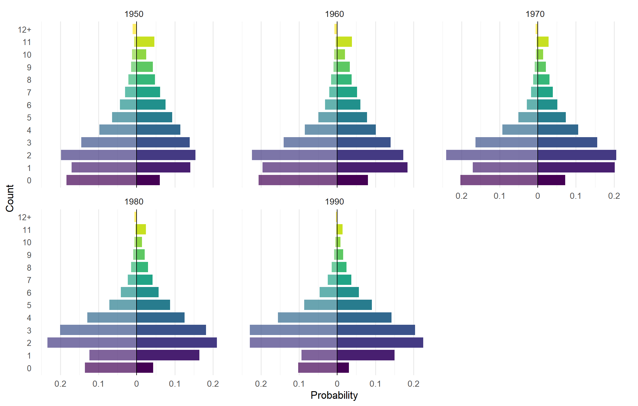
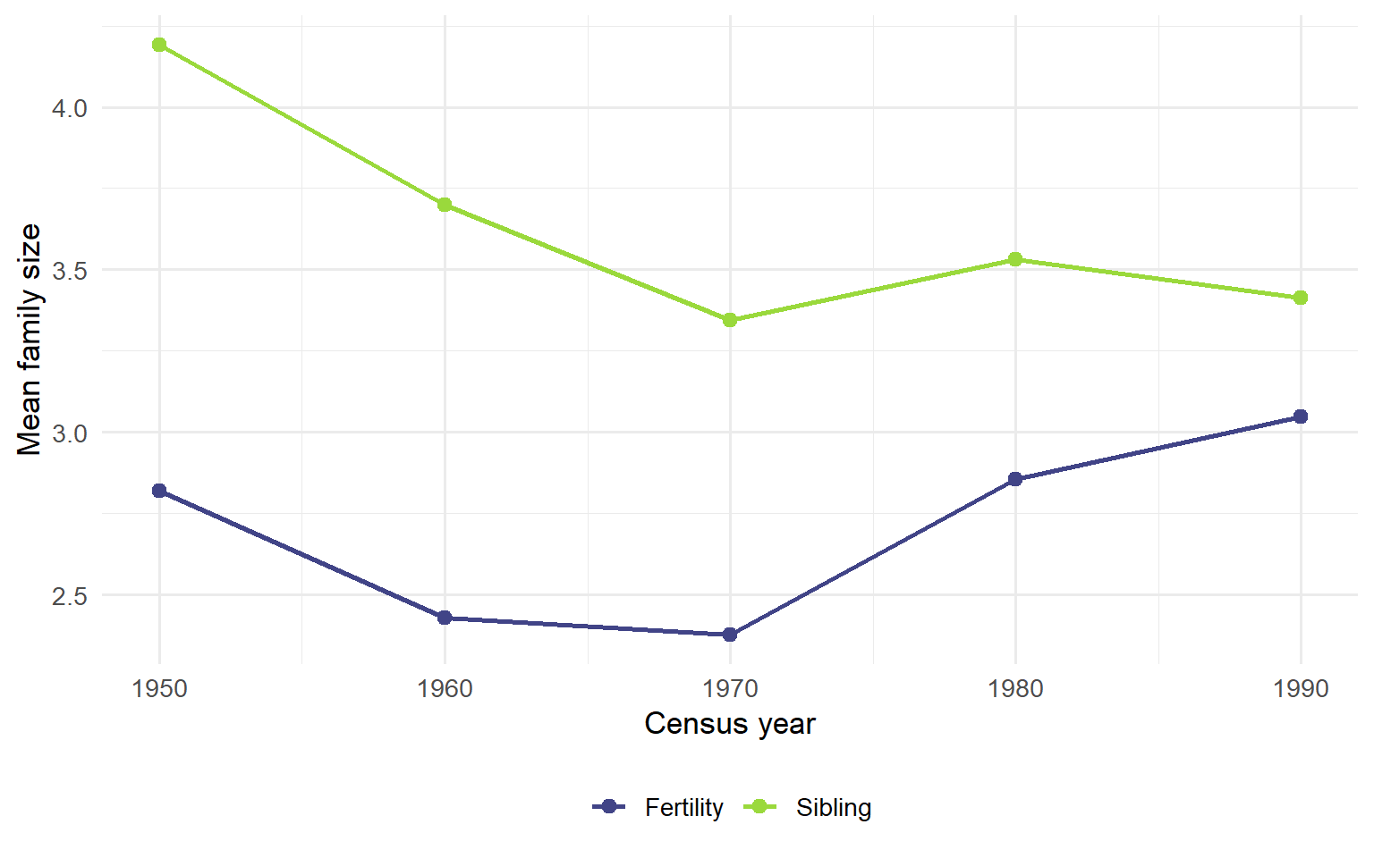
1.4 Visualise the fertility and sibling distributions across Census years

Code
plot_census_pmf <- function(fertility_df, sibling_df, max_count = 12) {
  pmf_df <- bind_rows(
    fertility_df %>%
      transmute(
        Year,
        Distribution = "Fertility",
        count = pmin(n_child, max_count)
      ),
    sibling_df %>%
      transmute(
        Year,
        Distribution = "Sibling",
        count = pmin(n_sib, max_count)
      )
  ) %>%
    count(Year, Distribution, count, name = "n_counts") %>%
    group_by(Year, Distribution) %>%
    mutate(prob = n_counts / sum(n_counts)) %>%
    ungroup()
  
  count_levels <- 0:max_count
  count_labels <- as.character(count_levels)
  count_labels[length(count_labels)] <- paste0(max_count, "+")
  
  pmf_df %>%
    mutate(
      signed_prob = if_else(Distribution == "Fertility", -prob, prob),
      count_cat = factor(count, levels = count_levels, labels = count_labels),
      Year = factor(Year)
    ) %>%
    ggplot(aes(x = count_cat, y = signed_prob, fill = count_cat, alpha = Distribution)) +
    geom_col(width = 0.82) +
    geom_hline(yintercept = 0, color = "black", linewidth = 0.4) +
    coord_flip() +
    facet_wrap(~ Year, ncol = 3) +
    scale_y_continuous(labels = function(x) abs(x)) +
    scale_fill_manual(values = viridis(length(count_levels), option = "D"), name = "Count") +
    scale_alpha_manual(values = c("Fertility" = 0.7, "Sibling" = 1), guide = "none") +
    labs(
      #title = "Probability mass functions (PMF) of fertility and sibling distributions across years",
      x = "Count",
      y = "Probability",
      # caption = "Left: Fertility distribution; Right: Sibling distribution"
    ) +
    theme_minimal(base_size = 13) +
    theme(
      plot.title = element_text(size = 14, hjust = 0.5),
      axis.text.y = element_text(size = 10),
      plot.caption = element_text(face = "bold", size = 10),
      legend.position = "none",
      panel.grid.major.y = element_blank(),
      panel.grid.minor.y = element_blank()
    )
}

plot_census_pmf(fertility_data, sib_data)

Code
ggsave(file = file.path(output_path, "census_fertility_sibling_pmf.pdf"), width = 11, height = 7)
Code
mean_across_years <- bind_rows(
  fertility_data %>%
    group_by(Year) %>%
    summarise(
      Distribution = "Fertility",
      Mean = mean(n_child),
      .groups = "drop"
    ),
  sib_data %>%
    group_by(Year) %>%
    summarise(
      Distribution = "Sibling",
      Mean = mean(n_sib),
      .groups = "drop"
    )
)

mean_across_years %>%
  ggplot(aes(x = Year, y = Mean, color = Distribution, group = Distribution)) +
  geom_line(linewidth = 1) +
  geom_point(size = 2.5) +
  scale_x_continuous(breaks = sort(unique(mean_across_years$Year))) +
  scale_color_manual(
    values = fertility_sibling_palette,
    name = NULL
  ) +
  labs(
    # title = "Mean Fertility and Sibling Counts Across Census Years",
    x = "Census year",
    y = "Mean family size"
  ) +
  theme_minimal(base_size = 13) +
  theme(
    plot.title = element_text(size = 14, hjust = 0.5),
    legend.position = "bottom"
  )

Code
ggsave(file = file.path(output_path, "mean_fertility_sibling_across_years.pdf"), width = 8, height = 5)

2 Family structure modelling

Here we establish statistical models for the fertility distribution and sibling distribution. The fertility distribution describes the number of children per family, while the sibling distribution describes the number of siblings per person.

2.1 Fertility distribution

We model the number of children per family using a Poisson distribution and a zero inflated negative binomial distribution (ZINB), respectively.

2.1.1 Poisson distribution

The Poisson distribution is a common model for count data, particularly when the mean and variance are equal. However, it may not be suitable for fertility data, which often exhibit zero-inflation and overdispersion (variance greater than the mean). The Poisson distribution with mean fertility (\(\mu\)) is defined as: for a count \(k \geq 0\), \[P(num_{child}=k)=e^{-\mu}\frac{\mu^k}{k!},\] denoted by \(Poisson(\mu)\). The mean and variance of \(Poisson(\mu)\) are both \(\mu\).

2.1.2 Zero inflated negative binomial distribution

The zero inflated negative binomial distribution with parameters mean fertility (\(\mu\)), dispersion/size (\(\theta\)), and zero‑inflation probability (\(\pi_0\))—denoted as \(ZINB(\mu, \theta, \pi_0)\)—is defined as: for a count \(k \geq 0\), \[P(num_{child}=k)=\begin{cases} \pi_0 + (1-\pi_0)p^{\theta} & \text{if } k=0, \\ (1-\pi_0)\binom{k+\theta-1}{k}(1-p)^k p ^{\theta} & \text{if } k \geq 1, \end{cases}\] where \(p = \frac{\theta}{\mu+\theta}\) represents the success probability of the negative binomial distribution.

According to the definition of the negative binomial distribution, the mean and variance of \(NB(\mu,\theta)\) are given by \(\mu\) and \(\mu + \frac{\mu^2}{\theta}\), respectively. Therefore, the mean and variance of \(ZINB(\mu, \theta, \pi_0)\) are defined by \(\mu(1-\pi_0)\) and \(\mu(1-\pi_0) + \frac{\mu^2(1-\pi_0)}{\theta}+\mu^2\pi_0(1-\pi_0)\), respectively.

2.2 Sibling distribution

The sibling distribution can be derived from the fertility distribution. For any count \(k \geq 0\), the probability that an individual has \(k\) siblings is proportional to the probability that their mother has \(k+1\) children, multiplied by the number of ways the individual could be one of those children. Therefore, the sibling distribution satisfies: \[P(num_{sib}=k) \propto (k+1)P(num_{child}=k+1).\]

2.2.1 Derivation of sibling distribution

If the fertility distribution is \(Poisson(\mu)\), then the sibling distribution is given by: for a count \(k \geq 0\), \[P(num_{sib}=k) \propto (k+1)e^{-\mu}\frac{\mu^{k+1}}{(k+1)!} = e^{-\mu}\frac{\mu^{k+1}}{k!}\propto e^{-\mu}\frac{\mu^k}{k!},\] which is also a Poisson distribution with mean \(\mu\).

If the fertility distribution is \(ZINB(\mu, \theta, \pi_0)\), then the sibling distribution is given by: for a count \(k \geq 0\), \[\begin{align*} P(num_{sib}=k) & \propto (1-\pi_0)(k+1)\binom{k+\theta}{k+1}(1-p)^{k+1} p^{\theta} \\ & = (1-\pi_0)(k+1)\frac{(k+\theta)!}{(k+1)!(\theta-1)!}(1-p)^{k+1} p^{\theta} \\ & \propto \frac{\theta(1-p)}{p} \frac{(k+\theta)!}{k!\theta!}(1-p)^k p^{\theta+1} \\ & \propto \binom{k+\theta}{k}(1-p)^k p^{\theta+1}, \\ \end{align*}\] where \(p = \frac{\theta}{\mu+\theta}\). Therefore, the sibling distribution is a negative binomial distribution with parameters mean fertility (\(\frac{\mu(\theta+1)}{\theta}\)), dispersion/size (\(\theta+1\)), denoted as \(NB(\frac{\mu(\theta+1)}{\theta}, \theta+1)\). The variance is \(\frac{\mu(\theta+1)}{\theta} + \frac{\mu^2(\theta+1)}{\theta^2}\).

3 Model fitting

3.1 Fit the Poisson and ZINB models

Code
fit_fert <- function(dat) {
  ## Poisson model
  pois <- glm(n_child ~ 1, family = poisson, data = dat)
  
  ## Zero‑inflated negative binomial model
  zinb <- zeroinfl(n_child ~ 1 | 1, data = dat, dist = "negbin")
  
  tibble(
    Model = c("Poisson", "ZINB"),
    mu    = c(exp(coef(pois)[1]),                    ## log‑link → exp() gives mean
              exp(zinb$coefficients$count[1])),
    size  = c(Inf,                                   ## dispersion θ; Inf = Poisson
              zinb$theta),
    pi0   = c(0,                                      ## zero‑inflation prob.
              plogis(zinb$coefficients$zero[1]))
  )
}

param_fert <- fertility_data %>%
  group_by(Year) %>%
  group_modify(~ fit_fert(.x)) %>%
  ungroup()

# Write the fitted parameters so downstream notebooks read them instead of
# hard-coding the values.
write.csv(param_fert, file.path(output_path, "fertility_parameters.csv"), row.names = FALSE)

3.2 Estimated fertility parameters

Code
kable(param_fert, digits = 3, caption = "Fertility‑model parameter estimates for women aged 50‑59 (1950, 1960, 1970, 1980, 1990)")
Fertility‑model parameter estimates for women aged 50‑59 (1950, 1960, 1970, 1980, 1990)
Year Model mu size pi0
1950 Poisson 2.818 Inf 0.000
1950 ZINB 2.943 2.372 0.043
1960 Poisson 2.429 Inf 0.000
1960 ZINB 2.458 2.088 0.012
1970 Poisson 2.377 Inf 0.000
1970 ZINB 2.547 3.578 0.067
1980 Poisson 2.855 Inf 0.000
1980 ZINB 3.036 6.947 0.060
1990 Poisson 3.047 Inf 0.000
1990 ZINB 3.224 19.792 0.055

3.3 Compare the mean and variance from the models and data

Code
cal_mean_var <- function(model, mu, size, pi0) {
  if (model == "Poisson") {
    mean_fert = mu
    var_fert  = mu
    mean_sib = mu
    var_sib  = mu
  } else if (model == "ZINB") {
    mean_fert = mu * (1 - pi0)
    var_fert  = mu * (1 - pi0) + (mu^2 * (1 - pi0) / size) + (mu^2 * pi0 * (1 - pi0))
    mean_sib = mu * ((size + 1) / size)
    var_sib  = mu * ((size + 1) / size) + (mu^2 * ((size + 1) / size) / size)
  }
  
  tibble(
    Model = model,
    Mean_Fertility = mean_fert,
    Variance_Fertility = var_fert,
    Mean_Sibling = mean_sib,
    Variance_Sibling = var_sib
  )
}

mean_var_fitted <- param_fert %>%
  rowwise(Year, Model) %>%
  reframe(cal_mean_var(Model, mu, size, pi0)) %>%
  ungroup()

mean_var_data <- bind_rows(
  fertility_data %>%
    group_by(Year) %>%
    summarise(
      distribution = "fertility",
      mean_data = mean(n_child),
      variance_data = var(n_child),
      .groups = "drop"
    ),
  sib_data %>%
    group_by(Year) %>%
    summarise(
      distribution = "sibling",
      mean_data = mean(n_sib),
      variance_data = var(n_sib),
      .groups = "drop"
    )
)

mean_var_model <- mean_var_fitted %>%
  transmute(
    Year,
    Model = tolower(Model),
    mean_fertility = Mean_Fertility,
    variance_fertility = Variance_Fertility,
    mean_sibling = Mean_Sibling,
    variance_sibling = Variance_Sibling
  ) %>%
  pivot_longer(
    cols = c(mean_fertility, variance_fertility, mean_sibling, variance_sibling),
    names_to = c(".value", "distribution"),
    names_pattern = "(mean|variance)_(fertility|sibling)"
  ) %>%
  pivot_wider(
    names_from = Model,
    values_from = c(mean, variance),
    names_glue = "{.value}_{Model}"
  )

mean_var <- mean_var_data %>%
  left_join(mean_var_model, by = c("distribution", "Year")) %>%
  dplyr::select(
    distribution,
    Year,
    mean_data,
    mean_poisson,
    mean_zinb,
    variance_data,
    variance_poisson,
    variance_zinb
  ) %>%
  arrange(distribution, Year)

write.csv(mean_var, file.path(output_path, "fertility_estimation.csv"), row.names = FALSE)

kable(mean_var, digits = 3, caption = "Mean and variance of fertility and sibling distributions from the fitted models and data.")
Mean and variance of fertility and sibling distributions from the fitted models and data.
distribution Year mean_data mean_poisson mean_zinb variance_data variance_poisson variance_zinb
fertility 1950 2.818 2.818 2.818 6.689 2.818 6.668
fertility 1960 2.429 2.429 2.429 5.513 2.429 5.359
fertility 1970 2.377 2.377 2.377 4.675 2.377 4.473
fertility 1980 2.855 2.855 2.855 4.787 2.855 4.620
fertility 1990 3.047 3.047 3.047 4.160 3.047 4.083
sibling 1950 4.192 2.818 4.184 8.891 2.818 9.376
sibling 1960 3.699 2.429 3.635 8.515 2.429 7.915
sibling 1970 3.344 2.377 3.259 7.057 2.377 5.579
sibling 1980 3.532 2.855 3.473 6.346 2.855 4.991
sibling 1990 3.412 3.047 3.387 5.026 3.047 3.938

3.4 Model evaluation

Based on the table of mean and variance, we can see that the fertility data exhibits overdispersion (variance greater than mean). The Poisson Model assumes equal mean and variance, which does not fit the data well. The ZINB Model accounts for overdispersion and zero-inflation, providing a better fit to the data. The ZINB model’s mean and variance estimates for both fertility and sibling distributions align more closely with the observed data.

4 Simulations of fertility and sibling distributions

In this section, we simulate the fertility and sibling counts based on the Poisson and ZINB distributions, respectively. We then compare the empirical mean and variance of the simulated sibling data with the theoretical values derived from Section 2.

4.1 Simulate the fertility and sibling counts

Code
simulate_fert_sib <- function(model, mu, size, pi0, n_sim = 20000, max_kids = 12) {
  if (model == "Poisson") {
    # Simulate fertility counts from Poisson distribution
    fert_counts <- pmin(rpois(n_sim, lambda = mu), max_kids)
  } else if (model == "ZINB") {
    # Simulate fertility counts from ZINB distribution
    fert_counts <- ifelse(runif(n_sim) < pi0, 0, pmin(rnbinom(n_sim, size, mu = mu), max_kids))
  }
  
  # Simulate sibling counts based on fertility counts
  fert_counts_tibble <- tibble(fert_counts = fert_counts)
  sib_counts_tibble <- fert_counts_tibble %>%
    filter(fert_counts > 0) %>%
    tidyr::uncount(fert_counts, .remove = FALSE) %>%
    mutate(sib_counts = fert_counts - 1)
  sib_counts <- sib_counts_tibble$sib_counts
  
  list(
    model = model,
    fert_counts = fert_counts,
    sib_counts = sib_counts
  )
}

4.2 Compare sibling counts from simulations with theoretical values

We run simulations for fertility means of 1.5, 2.0, 2.5, 3.0, 3.5, and 4.0 for both Poisson and ZINB models. Additionally, in ZINB models, we set the dispersion parameter \(\theta\) to 4, and the zero-inflation probability \(\pi_0\) to 0.05.

We compare the empirical mean and variance of sibling counts from the simulated data with the theoretical values. The comparison shows that the theoretical values align closely with the simulated results, confirming the correctness of our derivation.

Code
means = c(1.5, 2.0, 2.5, 3.0, 3.5, 4.0)
size = 4
pi0 = 0.05

cal_mean_var_simulated <- function(sim_data) {
  sib_counts <- sim_data$sib_counts
  
  mean_sib = mean(sib_counts)
  var_sib = var(sib_counts)
  
  tibble(
    Mean_Sibling = mean_sib,
    Variance_Sibling = var_sib
  )
}

# Poisson Model
simulated_poisson <- lapply(means, function(mu) {
  simulate_fert_sib("Poisson", mu, Inf, 0)
})

simulated_poisson_results <- lapply(simulated_poisson, cal_mean_var_simulated) %>% bind_rows() %>%
  mutate(Fertility_Parameter = sapply(means, function(mu) paste0("Fertility Mean = ", mu)),
         Value_Type = "Simulated Poisson") %>% dplyr::select(Fertility_Parameter, Value_Type, everything())
threo_possion_results <- tibble(
  Fertility_Parameter = sapply(means, function(mu) paste0("Fertility Mean = ", mu)),
  Value_Type = "Theoretical Poisson",
  Mean_Sibling = means,
  Variance_Sibling = means
)

poisson_results <- bind_rows(simulated_poisson_results, threo_possion_results) %>%
  arrange(Fertility_Parameter) %>%
  mutate(Value_Type = factor(Value_Type, levels = c("Theoretical Poisson", "Simulated Poisson")))

kable(poisson_results, digits = 3, caption = "Mean and Variance of Sibling counts from simulations and theoretical values based on Poisson distribution.")
Mean and Variance of Sibling counts from simulations and theoretical values based on Poisson distribution.
Fertility_Parameter Value_Type Mean_Sibling Variance_Sibling
Fertility Mean = 1.5 Simulated Poisson 1.505 1.572
Fertility Mean = 1.5 Theoretical Poisson 1.500 1.500
Fertility Mean = 2 Simulated Poisson 1.991 1.998
Fertility Mean = 2 Theoretical Poisson 2.000 2.000
Fertility Mean = 2.5 Simulated Poisson 2.514 2.471
Fertility Mean = 2.5 Theoretical Poisson 2.500 2.500
Fertility Mean = 3 Simulated Poisson 2.989 2.976
Fertility Mean = 3 Theoretical Poisson 3.000 3.000
Fertility Mean = 3.5 Simulated Poisson 3.486 3.480
Fertility Mean = 3.5 Theoretical Poisson 3.500 3.500
Fertility Mean = 4 Simulated Poisson 3.982 3.906
Fertility Mean = 4 Theoretical Poisson 4.000 4.000
Code
# ZINB Model
simulated_zinb <- lapply(means, function(mu) {
  simulate_fert_sib("ZINB", mu/(1-pi0), size, pi0)
})
simulated_zinb_results <- lapply(simulated_zinb, cal_mean_var_simulated) %>% bind_rows() %>%
  mutate(Fertility_Parameter = sapply(means, function(mu) paste0("Fertility Mean = ", mu)),
         Value_Type = "Simulated ZINB") %>% dplyr::select(Fertility_Parameter, Value_Type, everything())
mean_var_zinb <- lapply(means, function(mu) cal_mean_var("ZINB", mu/(1-pi0), size, pi0)) %>% bind_rows()
threo_zinb_results <- tibble(
  Fertility_Parameter = sapply(means, function(mu) paste0("Fertility Mean = ", mu)),
  Value_Type = "Theoretical ZINB",
  Mean_Sibling = mean_var_zinb$Mean_Sibling,
  Variance_Sibling = mean_var_zinb$Variance_Sibling
)

zinb_results <- bind_rows(simulated_zinb_results, threo_zinb_results) %>%
  arrange(Fertility_Parameter) %>%
  mutate(Value_Type = factor(Value_Type, levels = c("Theoretical ZINB", "Simulated ZINB")))

kable(zinb_results, digits = 3, caption = "Mean and Variance of Sibling counts from simulations and theoretical values based on ZINB distribution.")
Mean and Variance of Sibling counts from simulations and theoretical values based on ZINB distribution.
Fertility_Parameter Value_Type Mean_Sibling Variance_Sibling
Fertility Mean = 1.5 Simulated ZINB 1.930 2.751
Fertility Mean = 1.5 Theoretical ZINB 1.974 2.753
Fertility Mean = 2 Simulated ZINB 2.590 3.773
Fertility Mean = 2 Theoretical ZINB 2.632 4.017
Fertility Mean = 2.5 Simulated ZINB 3.271 5.266
Fertility Mean = 2.5 Theoretical ZINB 3.289 5.454
Fertility Mean = 3 Simulated ZINB 3.915 6.461
Fertility Mean = 3 Theoretical ZINB 3.947 7.064
Fertility Mean = 3.5 Simulated ZINB 4.555 7.676
Fertility Mean = 3.5 Theoretical ZINB 4.605 8.847
Fertility Mean = 4 Simulated ZINB 5.031 8.304
Fertility Mean = 4 Theoretical ZINB 5.263 10.803

4.3 Visualize sibling distributions

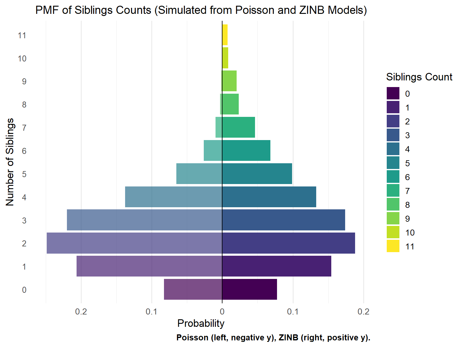
We generate discrete probability distributions for sibling counts based on both Poisson and ZINB models, with the y-axis representing the number of siblings and the x-axis representing the probability of having that many siblings. The fertility mean is set to 2.5, and the ZINB model has a dispersion parameter of 4 and a zero-inflation probability of 0.05.
Code
library(viridisLite)

plot_pmf <- function(pmf_df) {
  cats = sort(unique(pmf_df$sib_counts))
  n_cat <- length(cats)
  color_palette <- viridis(n_cat, option = "D")
  df <- pmf_df %>%
    mutate(y = ifelse(Model == "Poisson", -prob, prob),
           count_cat = factor(sib_counts, levels = cats))
  ggplot(df, aes(x = count_cat, y = y, fill = count_cat, alpha = Model)) +
    geom_col() +
    geom_hline(yintercept = 0, color = "black", size = 0.5) +
    coord_flip() +
    scale_y_continuous(labels = function(x) abs(x)) +
    scale_fill_manual(values = color_palette, name = "Siblings Count") +
    scale_alpha_manual(values = c("Poisson" = 0.7, "ZINB" = 1), guide = "none") +
    labs(
      title = "PMF of Siblings Counts (Simulated from Poisson and ZINB Models)",
      x = "Number of Siblings",
      y = "Probability",
      caption = "Poisson (left, negative y), ZINB (right, positive y)."
    ) +
    theme_minimal(base_size = 13) +
    theme(
      plot.title = element_text(size = 14, hjust = 0.5),
      axis.text.y = element_text(size = 10),
      plot.caption = element_text(face = "bold", size = 10),
      legend.position = "right",
      panel.grid.major.y = element_blank(),
      panel.grid.minor.y = element_blank()
    )
}
Code
# fertility parameters
mean = 2.5
size = 4
pi0 = 0.05
max_sibs = 12

# simulated data for fertility mean 2.5
simulated_data <- bind_rows(
  tibble(sib_counts = simulate_fert_sib("Poisson", mean, Inf, 0)$sib_counts) %>%
    mutate(Model = "Poisson"),
  tibble(sib_counts = simulate_fert_sib("ZINB", mean/(1-pi0), size, pi0)$sib_counts) %>%
    mutate(Model = "ZINB")
)

simulated_data$sib_counts <- ifelse(simulated_data$sib_counts > max_sibs, max_sibs, simulated_data$sib_counts)

pmf_data <- simulated_data %>%
  count(Model, sib_counts, name = "n_counts") %>%
  group_by(Model) %>%
  mutate(prob = n_counts / sum(n_counts)) %>%
  ungroup()

# write the pmf data to a csv file
write.csv(pmf_data, file = file.path(output_path, "pmf_sibling_counts.csv"), row.names = FALSE)
Code
plot_pmf(pmf_data)

Code
ggsave(file = file.path(output_path, "pmf_sibling_counts.png"), width = 8, height = 6, dpi = 500)
Code
sum(pmf_data$n_counts[pmf_data$Model == "Poisson"])
[1] 49982
Code
sum(pmf_data$n_counts[pmf_data$Model == "ZINB"])
[1] 50371
Code
pmf_data$n_counts[pmf_data$Model == "Poisson"] / sum(pmf_data$n_counts[pmf_data$Model == "Poisson"])
 [1] 0.0825897323 0.2063142731 0.2484894562 0.2197591133 0.1376495538
 [6] 0.0648233364 0.0260493778 0.0094433996 0.0032411668 0.0012004322
[11] 0.0004401585
Code
pmf_data$n_counts[pmf_data$Model == "ZINB"] / sum(pmf_data$n_counts[pmf_data$Model == "ZINB"])
 [1] 0.077743146 0.154295130 0.188143972 0.174068412 0.132913780 0.098985527
 [7] 0.068094737 0.046217069 0.023406325 0.020448274 0.008298426 0.007385202