Preprocessing IPUMS fertility data

Author

Tina Lasisi

Published

August 3, 2026

This notebook converts a restricted IPUMS USA extract into the aggregate fertility summaries used throughout the kincounts project, and documents the processing decisions. It makes two analytic contributions:

  1. Completed-fertility distributions by birth cohort — women aged 50–59 in each census from 1950 to 1990 (children ever born), the inputs used by the downstream fertility model and simulator.
  2. A common-universe analysis — a measurement of how those distributions change when the population that was asked the children-ever-born question shifts from ever-married women (1950–1960) to all women (1970–1990).

Because IPUMS USA policy restricts redistribution of raw microdata, only the aggregate CSVs in data/processed/ are committed; the raw extract stays local-only (ignored by Git via .gitignore). Processing code is collapsed by default; the sections below present the resulting figures and tables.

1 Data source and access

The source data are an IPUMS USA extract (a fixed-width *.dat.gz plus its *.xml DDI codebook) covering the 1950, 1960, 1970, 1980, and 1990 U.S. Census samples. The variables used are YEAR, PERWT, SEX, AGE, BIRTHYR, MARST, GQ, and CHBORN. The sample-line weight SLWT, the allocation flag QCHBORN, and the nativity/birthplace variables NATIVITY/BPL were not requested; their absence is discussed in the limitations.

Formal citation:

Steven Ruggles, Sarah Flood, Matthew Sobek, Daniel Backman, Grace Cooper, Julia A. Rivera Drew, Stephanie Richards, Renae Rodgers, Jonathan Schroeder, and Kari C.W. Williams. IPUMS USA: Version 16.0 [dataset]. Minneapolis, MN: IPUMS, 2025. https://doi.org/10.18128/D010.V16.0

To reproduce the raw-data step, create your own IPUMS USA extract with the same samples and variables, place the .dat.gz and .xml files in data/raw/, and render this notebook locally. Only the aggregate CSVs in data/processed/ should be committed.

2 Data processing

By default, the code below loads the committed aggregate CSVs in data/processed/ without looking for or opening the restricted raw IPUMS files. To rebuild those aggregates from a local raw extract, set KINCOUNTS_REBUILD_IPUMS=true for the render; only that explicit flag triggers raw parsing.

Code
# Packages for IPUMS parsing, data manipulation, CSV I/O, tables, and figures.
library(ipumsr)
library(dplyr)
library(tidyr)
library(readr)
library(knitr)
library(ggplot2)
library(viridisLite)

theme_set(theme_minimal(base_size = 12))

coverage_palette <- setNames(
  viridis(3, option = "D", begin = 0.12, end = 0.88),
  c("Ever-married, 1-in-6 sample line", "Ever-married women", "All women")
)
universe_palette <- setNames(
  viridis(2, option = "D", begin = 0.2, end = 0.85),
  c("All women", "Ever-married")
)
validation_palette <- setNames(
  viridis(2, option = "D", begin = 0.2, end = 0.85),
  c("Direct 1950", "Proxy (1960)")
)
main_series_color <- viridis(1, option = "D", begin = 0.55, end = 0.55)

# Resolve paths whether rendered from the project root or the analysis directory.
project_root <- if (dir.exists("data")) "." else ".."
raw_dir <- Sys.getenv("KINCOUNTS_RAW_DIR", file.path(project_root, "data", "raw"))
processed_dir <- file.path(project_root, "data", "processed")
dir.create(processed_dir, recursive = TRUE, showWarnings = FALSE)

processing_version <- "common_universe_v5"

# Variables parsed from the restricted person-level data when rebuilding.
analysis_vars <- c("YEAR", "PERWT", "SEX", "AGE", "BIRTHYR", "MARST", "GQ", "CHBORN")
ddi_display_vars <- analysis_vars

# Every aggregate file this notebook writes or expects to load.
output_inventory <- bind_rows(
  tibble(
    file = c(
      "ipums_preprocess_metadata.csv",
      "ipums_cohort_sample_sizes.csv",
      "ipums_fertility_counts_by_cohort.csv",
      "ipums_fertility_pmf_by_cohort.csv",
      "ipums_fertility_counts_by_cohort_weighted.csv",
      "ipums_fertility_pmf_by_cohort_weighted.csv",
      "validation_1950_direct_vs_proxy.csv",
      "validation_1950_direct_vs_proxy_pmf.csv",
      "ipums_age_cohort_validation.csv",
      "ipums_chborn_universe_by_cohort.csv",
      "ipums_cohort_fertility_checks.csv",
      "ipums_cohort_universe_summary.csv",
      "ipums_cohort_universe_pmf.csv",
      "ipums_universe_contrast_by_cohort.csv",
      "ipums_early_cohort_followup.csv"
    ),
    contents = c(
      "Processing version and rebuild timestamp.",
      "Main-series sample sizes by output cohort.",
      "Unweighted main-series fertility counts by cohort and child-count bucket.",
      "Unweighted main-series fertility PMF by cohort and child-count bucket.",
      "PERWT-weighted main-series fertility counts.",
      "PERWT-weighted main-series fertility PMF.",
      "Aggregate comparison of proxy 1950 and direct 1950 validation records.",
      "Child-count PMFs for proxy 1950 and direct 1950 validation records.",
      "Age range and derived birth-year span for each age-defined cohort source.",
      "Valid versus not-in-universe CHBORN counts by cohort source.",
      "Aggregate mean children and 12+ share by cohort source.",
      "Common-universe analysis: per decade-cohort x census x universe summary.",
      "Common-universe analysis: child-count PMFs per decade-cohort x census x universe.",
      "All-women vs ever-married contrast (mean shift, share-0 shift, TVD) by cohort.",
      "Early-cohort decomposition of universe vs mortality/decade effects."
    ),
    role = c(
      "Reproducibility check",
      "Downstream model input",
      "Downstream model input",
      "Downstream model input",
      "Sensitivity output",
      "Sensitivity output",
      "Validation output",
      "Validation output",
      "QA output",
      "QA output",
      "QA output",
      "Common-universe analysis",
      "Common-universe analysis",
      "Common-universe analysis",
      "Common-universe analysis"
    )
  ),
  tibble(
    file = paste0("fertility_pmf_", c(1950, 1960, 1970, 1980, 1990), ".csv"),
    contents = "One unweighted main-series fertility PMF for the named output year.",
    role = "Downstream simulator input"
  )
)

processed_files <- output_inventory$file
processed_paths <- file.path(processed_dir, processed_files)

force_rebuild <- tolower(Sys.getenv("KINCOUNTS_REBUILD_IPUMS", "false")) %in%
  c("true", "1", "yes")

dat_gz_file <- NA_character_
ddi_file <- NA_character_
has_raw_extract <- FALSE
if (force_rebuild) {
  dat_gz_files <- Sys.glob(file.path(raw_dir, "*.dat.gz"))
  ddi_files <- Sys.glob(file.path(raw_dir, "*.xml"))
  has_raw_extract <- length(dat_gz_files) == 1 && length(ddi_files) == 1
  if (!has_raw_extract) {
    stop(
      "KINCOUNTS_REBUILD_IPUMS=true requires exactly one .dat.gz and one .xml file in ",
      raw_dir,
      call. = FALSE
    )
  }
  dat_gz_file <- dat_gz_files
  ddi_file <- ddi_files
}

# Normal renders use the committed aggregate files. Rebuilding from the restricted
# person-level extract happens only when explicitly requested.
metadata_path <- file.path(processed_dir, "ipums_preprocess_metadata.csv")
metadata_current <- file.exists(metadata_path) &&
  identical(
    read_csv(metadata_path, show_col_types = FALSE)$processing_version[[1]],
    processing_version
  )
processed_complete <- all(file.exists(processed_paths)) && metadata_current
processed_current <- processed_complete

if (!force_rebuild && !processed_complete) {
  stop(
    "The processed CSV cache is incomplete or was built with an older processing version. ",
    "Use the committed data/processed files, or add the raw extract and render with ",
    "KINCOUNTS_REBUILD_IPUMS=true to rebuild.",
    call. = FALSE
  )
}

rebuild_processed <- force_rebuild

if (rebuild_processed) {
  # The DDI supplies the fixed-width layout and the value labels used below.
  ddi <- read_ipums_ddi(ddi_file)

  ddi_vars <- ipums_var_info(ddi)
  missing_vars <- setdiff(ddi_display_vars, ddi_vars$var_name)
  if (length(missing_vars) > 0) {
    stop(
      "The DDI is missing required variables: ",
      paste(missing_vars, collapse = ", "),
      call. = FALSE
    )
  }

  # Check that ipumsr can parse a few records using the DDI layout.
  parse_check <- read_ipums_micro(
    ddi,
    vars = analysis_vars,
    n_max = 5,
    data_file = dat_gz_file,
    verbose = FALSE
  )
  stopifnot(nrow(parse_check) == 5)
  rm(parse_check)

  # DDI variable positions (rendered in the appendix).
  ddi_variables <- ddi_vars %>%
    filter(var_name %in% ddi_display_vars) %>%
    arrange(match(var_name, ddi_display_vars)) %>%
    select(var_name, var_label, start, end, imp_decim)

  # DDI value labels that drive the coding rules (rendered in the coding section).
  value_labels <- bind_rows(lapply(c("SEX", "CHBORN", "MARST"), function(var) {
    labels <- ddi_vars$val_labels[[match(var, ddi_vars$var_name)]]
    mutate(labels, var_name = var, .before = 1)
  }))
} else {
  ddi_variables <- tibble(
    var_name = ddi_display_vars,
    var_label = "Raw DDI unavailable in processed-only render",
    start = NA_integer_,
    end = NA_integer_,
    imp_decim = NA_integer_
  )
  value_labels <- tibble(
    var_name = c("SEX", "SEX", "CHBORN", "CHBORN", "CHBORN", "CHBORN", "MARST", "MARST", "MARST"),
    val = c("1", "2", "0", "1", "13", "97-99", "1-5", "6", "9"),
    lbl = c(
      "Male",
      "Female",
      "N/A (not in universe)",
      "No children",
      "12 children; 12+ in 1960-1990",
      "Unknown, illegible, or missing",
      "Ever-married",
      "Never-married",
      "Blank/missing"
    )
  )
}

# Local filenames and cache state (rendered in the appendix).
file_summary <- tibble(
  item = c(
    "compressed_data_file",
    "ddi_codebook",
    "compressed_size_mib",
    "raw_extract_used",
    "processed_outputs_current",
    "rebuild_from_raw"
  ),
  value = c(
    if (has_raw_extract) basename(dat_gz_file) else NA_character_,
    if (has_raw_extract) basename(ddi_file) else NA_character_,
    if (has_raw_extract) round(file.info(dat_gz_file)$size / 1024^2, 1) else NA_real_,
    has_raw_extract,
    processed_current,
    rebuild_processed
  )
)

output_path <- if (dir.exists("output")) "output" else file.path("..", "output")
Code
if (rebuild_processed) {
  # Parse only the variables used for filtering, cohort assignment, weights,
  # and fertility counts.
  ipums_data <- read_ipums_micro(
    ddi,
    vars = analysis_vars,
    data_file = dat_gz_file,
    verbose = FALSE
  ) %>%
    mutate(across(all_of(analysis_vars), as.numeric))

  # --- Main series: age-first cohort assignment (membership defined by AGE within
  # a census). The 1950 cohort is a proxy from women aged 60-69 in 1960; direct
  # 1950 (women 50-59 in 1950) is held out for validation. Birth-year spans are
  # derived afterwards for labeling only.
  cohort_records <- ipums_data %>%
    filter(SEX == 2) %>%
    mutate(
      source_year = YEAR,
      cohort_source = case_when(
        YEAR == 1950 & between(AGE, 50, 59) ~ "direct_1950_validation",
        YEAR == 1960 & between(AGE, 60, 69) ~ "proxy_1950",
        YEAR == 1960 & between(AGE, 50, 59) ~ "main_1960",
        YEAR == 1970 & between(AGE, 50, 59) ~ "main_1970",
        YEAR == 1980 & between(AGE, 50, 59) ~ "main_1980",
        YEAR == 1990 & between(AGE, 50, 59) ~ "main_1990",
        TRUE ~ NA_character_
      ),
      Year = case_when(
        cohort_source %in% c("proxy_1950", "direct_1950_validation") ~ 1950,
        cohort_source == "main_1960" ~ 1960,
        cohort_source == "main_1970" ~ 1970,
        cohort_source == "main_1980" ~ 1980,
        cohort_source == "main_1990" ~ 1990,
        TRUE ~ NA_real_
      ),
      series = case_when(
        cohort_source == "direct_1950_validation" ~ "validation",
        !is.na(cohort_source) ~ "main",
        TRUE ~ NA_character_
      ),
      valid_chborn = CHBORN > 0 & CHBORN < 97,
      n_child = if_else(valid_chborn, pmin(CHBORN - 1, 12), NA_real_)
    ) %>%
    filter(!is.na(cohort_source))

  cohort_composition <- cohort_records %>%
    group_by(series, cohort_source, source_year, Year) %>%
    summarise(
      n_records = n(),
      age_min = min(AGE, na.rm = TRUE),
      age_max = max(AGE, na.rm = TRUE),
      birthyr_min = min(BIRTHYR[BIRTHYR > 1800], na.rm = TRUE),
      birthyr_max = max(BIRTHYR[BIRTHYR > 1800], na.rm = TRUE),
      .groups = "drop"
    ) %>%
    mutate(cohort = paste0(birthyr_min, "-", birthyr_max)) %>%
    arrange(Year, source_year, cohort_source)

  cohort_records <- cohort_records %>%
    left_join(select(cohort_composition, cohort_source, cohort), by = "cohort_source")

  age_cohort_validation <- cohort_composition
  completed_fertility <- cohort_records
  valid_completed_fertility <- completed_fertility %>% filter(valid_chborn)
  main_fertility <- valid_completed_fertility %>% filter(series == "main")
  validation_1950 <- valid_completed_fertility %>%
    filter(cohort_source %in% c("proxy_1950", "direct_1950_validation"))

  # How much data the CHBORN validity rule excludes, by cohort source.
  chborn_universe <- completed_fertility %>%
    count(cohort_source, source_year, Year, cohort, valid_chborn, name = "n_records") %>%
    pivot_wider(
      names_from = valid_chborn,
      values_from = n_records,
      names_prefix = "valid_chborn_",
      values_fill = 0
    ) %>%
    mutate(
      total_records = valid_chborn_FALSE + valid_chborn_TRUE,
      valid_share = valid_chborn_TRUE / total_records
    ) %>%
    arrange(Year, source_year, cohort_source)

  cohort_means <- valid_completed_fertility %>%
    group_by(cohort_source, series, source_year, Year, cohort) %>%
    summarise(
      n_women = n(),
      n_women_weighted = sum(PERWT, na.rm = TRUE),
      mean_children = mean(n_child),
      mean_children_weighted = weighted.mean(n_child, PERWT, na.rm = TRUE),
      share_12plus = mean(n_child == 12),
      .groups = "drop"
    ) %>%
    arrange(series, Year, source_year, cohort_source)

  fertility_counts <- main_fertility %>%
    count(Year, cohort, n_child, name = "n_women") %>%
    arrange(Year, n_child)

  fertility_counts_weighted <- main_fertility %>%
    group_by(Year, cohort, n_child) %>%
    summarise(n_women_weighted = sum(PERWT, na.rm = TRUE), .groups = "drop") %>%
    arrange(Year, n_child)

  fertility_pmf <- fertility_counts %>%
    group_by(Year, cohort) %>%
    mutate(probability = n_women / sum(n_women)) %>%
    ungroup() %>%
    transmute(Year, cohort, children = n_child, probability)

  fertility_pmf_weighted <- fertility_counts_weighted %>%
    group_by(Year, cohort) %>%
    mutate(probability_weighted = n_women_weighted / sum(n_women_weighted)) %>%
    ungroup() %>%
    transmute(Year, cohort, children = n_child, probability_weighted)

  cohort_sample_sizes <- main_fertility %>%
    group_by(Year, cohort) %>%
    summarise(
      n_women = n(),
      n_women_weighted = sum(PERWT, na.rm = TRUE),
      .groups = "drop"
    ) %>%
    arrange(Year)

  validation_1950_summary <- validation_1950 %>%
    group_by(cohort_source) %>%
    summarise(
      source_year = first(source_year),
      output_year = first(Year),
      n_women = n(),
      n_women_weighted = sum(PERWT, na.rm = TRUE),
      mean_children = mean(n_child),
      mean_children_weighted = weighted.mean(n_child, PERWT, na.rm = TRUE),
      share_12plus = mean(n_child == 12),
      .groups = "drop"
    ) %>%
    arrange(cohort_source)

  validation_1950_pmf <- validation_1950 %>%
    count(cohort_source, n_child, name = "n_women") %>%
    left_join(
      validation_1950 %>%
        group_by(cohort_source, n_child) %>%
        summarise(n_women_weighted = sum(PERWT, na.rm = TRUE), .groups = "drop"),
      by = c("cohort_source", "n_child")
    ) %>%
    group_by(cohort_source) %>%
    mutate(
      probability = n_women / sum(n_women),
      probability_weighted = n_women_weighted / sum(n_women_weighted)
    ) %>%
    ungroup() %>%
    arrange(cohort_source, n_child)

  # --- Common-universe analysis (separate frame; the main series is untouched).
  # Follow decade birth cohorts across the 1960-1990 censuses and, where the whole
  # cohort has reached age 50+, contrast the children-ever-born distribution under
  # two universes: all women vs ever-married. This isolates the effect of the
  # universe shift (1950/1960 asked only ever-married women; 1970-1990 all women).
  # MARST: 1-5 = ever-married, 6 = never-married, 9 = blank/missing (kept in the
  # all-women universe but excluded from the ever-married subset).
  band_records <- ipums_data %>%
    filter(SEX == 2, between(YEAR, 1960, 1990), between(BIRTHYR, 1890, 1939)) %>%
    mutate(
      band_start = 10L * (BIRTHYR %/% 10L),
      birth_band = paste0(band_start, "-", band_start + 9L),
      universe_year = YEAR,
      # Keep only cells where the whole decade cohort has reached age 50+.
      cohort_complete = (universe_year - (band_start + 9L)) >= 50L,
      valid_chborn = CHBORN > 0 & CHBORN < 97,
      n_child = if_else(valid_chborn, pmin(CHBORN - 1, 12), NA_real_),
      marital = case_when(
        MARST %in% 1:5 ~ "ever_married",
        MARST == 6 ~ "never_married",
        TRUE ~ "unknown"
      ),
      gq_household = GQ %in% c(1, 2, 5)
    ) %>%
    filter(cohort_complete, valid_chborn)

  band_long <- bind_rows(
    band_records %>% mutate(universe = "all_women"),
    band_records %>% filter(marital == "ever_married") %>% mutate(universe = "ever_married")
  )

  band_summary <- band_long %>%
    group_by(birth_band, universe_year, universe) %>%
    summarise(
      age_min = min(AGE),
      age_max = max(AGE),
      n_women = n(),
      n_women_weighted = sum(PERWT),
      mean_children = mean(n_child),
      mean_children_weighted = weighted.mean(n_child, PERWT),
      var_children = var(n_child),
      share_0 = mean(n_child == 0),
      share_12plus = mean(n_child == 12),
      gq_household_share = mean(gq_household),
      .groups = "drop"
    ) %>%
    arrange(birth_band, universe_year, universe)

  band_pmf <- band_long %>%
    count(birth_band, universe_year, universe, n_child, name = "n_women") %>%
    left_join(
      band_long %>%
        group_by(birth_band, universe_year, universe, n_child) %>%
        summarise(n_women_weighted = sum(PERWT), .groups = "drop"),
      by = c("birth_band", "universe_year", "universe", "n_child")
    ) %>%
    group_by(birth_band, universe_year, universe) %>%
    mutate(
      probability = n_women / sum(n_women),
      probability_weighted = n_women_weighted / sum(n_women_weighted)
    ) %>%
    ungroup() %>%
    arrange(birth_band, universe_year, universe, n_child)

  # Within-census contrast. The two universes coincide by construction before 1970
  # (never-married women were not in the CHBORN universe), so the contrast is
  # meaningful only for universe_year >= 1970.
  universe_contrast <- band_summary %>%
    select(birth_band, universe_year, universe, n_women, mean_children, var_children, share_0) %>%
    pivot_wider(
      names_from = universe,
      values_from = c(n_women, mean_children, var_children, share_0)
    ) %>%
    mutate(
      mean_shift = mean_children_all_women - mean_children_ever_married,
      share0_shift = share_0_all_women - share_0_ever_married,
      pct_never_married = 1 - n_women_ever_married / n_women_all_women
    )

  tvd_table <- band_pmf %>%
    select(birth_band, universe_year, universe, n_child, probability, probability_weighted) %>%
    pivot_wider(
      names_from = universe,
      values_from = c(probability, probability_weighted),
      values_fill = 0
    ) %>%
    group_by(birth_band, universe_year) %>%
    summarise(
      tvd = 0.5 * sum(abs(probability_all_women - probability_ever_married)),
      tvd_weighted = 0.5 * sum(abs(probability_weighted_all_women - probability_weighted_ever_married)),
      .groups = "drop"
    )

  universe_contrast <- universe_contrast %>%
    left_join(tvd_table, by = c("birth_band", "universe_year")) %>%
    arrange(birth_band, universe_year)

  # Early-cohort decomposition: the two cohorts seen ever-married at completed
  # fertility (1960) and all-women later (1970). Split the gap into the universe
  # effect (same census, adding never-married women) and the mortality/decade
  # effect (same ever-married universe, older age).
  pick_mean <- function(b, y, u) {
    v <- band_summary$mean_children[
      band_summary$birth_band == b &
        band_summary$universe_year == y &
        band_summary$universe == u
    ]
    if (length(v) == 1) v else NA_real_
  }
  early_cohort_followup <- tibble(
    birth_band = c("1890-1899", "1900-1909"),
    completed_year = c(1960, 1960),
    later_year = c(1970, 1970)
  ) %>%
    mutate(
      completed_em_mean = mapply(function(b, y) pick_mean(b, y, "ever_married"), birth_band, completed_year),
      later_em_mean = mapply(function(b, y) pick_mean(b, y, "ever_married"), birth_band, later_year),
      later_all_mean = mapply(function(b, y) pick_mean(b, y, "all_women"), birth_band, later_year),
      universe_effect = later_all_mean - later_em_mean,
      mortality_effect = later_em_mean - completed_em_mean
    )

  # Self-check: the 1900-1909 / 1960 ever-married mean should be close to the main
  # 1960 series mean, and 1890-1899 / 1960 close to the proxy-1950 mean.
  message(
    "Self-check (common-universe vs main series): ",
    "1900-1909/1960 ever-married mean = ", round(pick_mean("1900-1909", 1960, "ever_married"), 3),
    " (main_1960 ~ 2.429); ",
    "1890-1899/1960 ever-married mean = ", round(pick_mean("1890-1899", 1960, "ever_married"), 3),
    " (proxy_1950 ~ 2.818)."
  )

  # Write the aggregate CSVs.
  write_csv(cohort_sample_sizes, file.path(processed_dir, "ipums_cohort_sample_sizes.csv"))
  write_csv(fertility_counts, file.path(processed_dir, "ipums_fertility_counts_by_cohort.csv"))
  write_csv(fertility_pmf, file.path(processed_dir, "ipums_fertility_pmf_by_cohort.csv"))
  write_csv(fertility_counts_weighted, file.path(processed_dir, "ipums_fertility_counts_by_cohort_weighted.csv"))
  write_csv(fertility_pmf_weighted, file.path(processed_dir, "ipums_fertility_pmf_by_cohort_weighted.csv"))
  write_csv(validation_1950_summary, file.path(processed_dir, "validation_1950_direct_vs_proxy.csv"))
  write_csv(validation_1950_pmf, file.path(processed_dir, "validation_1950_direct_vs_proxy_pmf.csv"))
  write_csv(age_cohort_validation, file.path(processed_dir, "ipums_age_cohort_validation.csv"))
  write_csv(chborn_universe, file.path(processed_dir, "ipums_chborn_universe_by_cohort.csv"))
  write_csv(cohort_means, file.path(processed_dir, "ipums_cohort_fertility_checks.csv"))
  write_csv(band_summary, file.path(processed_dir, "ipums_cohort_universe_summary.csv"))
  write_csv(band_pmf, file.path(processed_dir, "ipums_cohort_universe_pmf.csv"))
  write_csv(universe_contrast, file.path(processed_dir, "ipums_universe_contrast_by_cohort.csv"))
  write_csv(early_cohort_followup, file.path(processed_dir, "ipums_early_cohort_followup.csv"))
  write_csv(
    tibble(
      processing_version = processing_version,
      cohort_definition = "main series: age-defined cohorts (50-59; proxy-1950 from 60-69 in 1960; direct-1950 validation-only); CHBORN harmonized to 12+. Common-universe analysis: decade birth cohorts followed across 1960-1990 at completed ages, all-women vs ever-married (MARST 1-5).",
      rebuilt_at = as.character(Sys.time())
    ),
    file.path(processed_dir, "ipums_preprocess_metadata.csv")
  )

  fertility_pmf %>%
    group_split(Year) %>%
    lapply(function(dat) {
      year <- unique(dat$Year)
      write_csv(
        dat %>% transmute(children, probability),
        file.path(processed_dir, paste0("fertility_pmf_", year, ".csv"))
      )
    })

  rm(
    ipums_data, cohort_records, cohort_composition, completed_fertility,
    valid_completed_fertility, main_fertility, validation_1950,
    band_records, band_long, tvd_table
  )
} else {
  # Load the committed aggregates without reparsing restricted person-level data.
  rd <- function(f) read_csv(file.path(processed_dir, f), show_col_types = FALSE)
  cohort_sample_sizes <- rd("ipums_cohort_sample_sizes.csv")
  fertility_counts <- rd("ipums_fertility_counts_by_cohort.csv")
  fertility_pmf <- rd("ipums_fertility_pmf_by_cohort.csv")
  fertility_counts_weighted <- rd("ipums_fertility_counts_by_cohort_weighted.csv")
  fertility_pmf_weighted <- rd("ipums_fertility_pmf_by_cohort_weighted.csv")
  validation_1950_summary <- rd("validation_1950_direct_vs_proxy.csv")
  validation_1950_pmf <- rd("validation_1950_direct_vs_proxy_pmf.csv")
  age_cohort_validation <- rd("ipums_age_cohort_validation.csv")
  chborn_universe <- rd("ipums_chborn_universe_by_cohort.csv")
  cohort_means <- rd("ipums_cohort_fertility_checks.csv")
  band_summary <- rd("ipums_cohort_universe_summary.csv")
  band_pmf <- rd("ipums_cohort_universe_pmf.csv")
  universe_contrast <- rd("ipums_universe_contrast_by_cohort.csv")
  early_cohort_followup <- rd("ipums_early_cohort_followup.csv")
  preprocess_metadata <- rd("ipums_preprocess_metadata.csv")
  if (!identical(preprocess_metadata$processing_version[[1]], processing_version)) {
    stop(
      "Processed files were built with processing version ",
      preprocess_metadata$processing_version[[1]],
      "; expected ", processing_version,
      ". Re-render with KINCOUNTS_REBUILD_IPUMS=true.",
      call. = FALSE
    )
  }
}

# Confirm the complete aggregate output set is available after either branch.
written_files <- tibble(
  file = processed_files,
  status = if_else(file.exists(processed_paths), "available", "missing")
)
if (any(written_files$status == "missing")) {
  stop(
    "Missing processed files: ",
    paste(written_files$file[written_files$status == "missing"], collapse = ", "),
    call. = FALSE
  )
}
3 The children-ever-born question and its universe

CHBORN records the number of children ever born alive to a woman. It counts live births only — stillbirths are excluded, as are adopted children and stepchildren.

For a multi-decade comparison, the central complication is that who was asked the question — the variable’s universe — changed across censuses:

Census Universe (who was asked)
1950 ever-married women, and only the 1-in-6 sample line
1960 ever-married women
1970 all women age 15+
1980 all women age 15+
1990 all women age 15+

A woman not in the universe was not asked the question and has no recorded value (IPUMS code 00), which is distinct from a recorded count of zero. Such records are excluded from all fertility distributions. Two consequences follow.

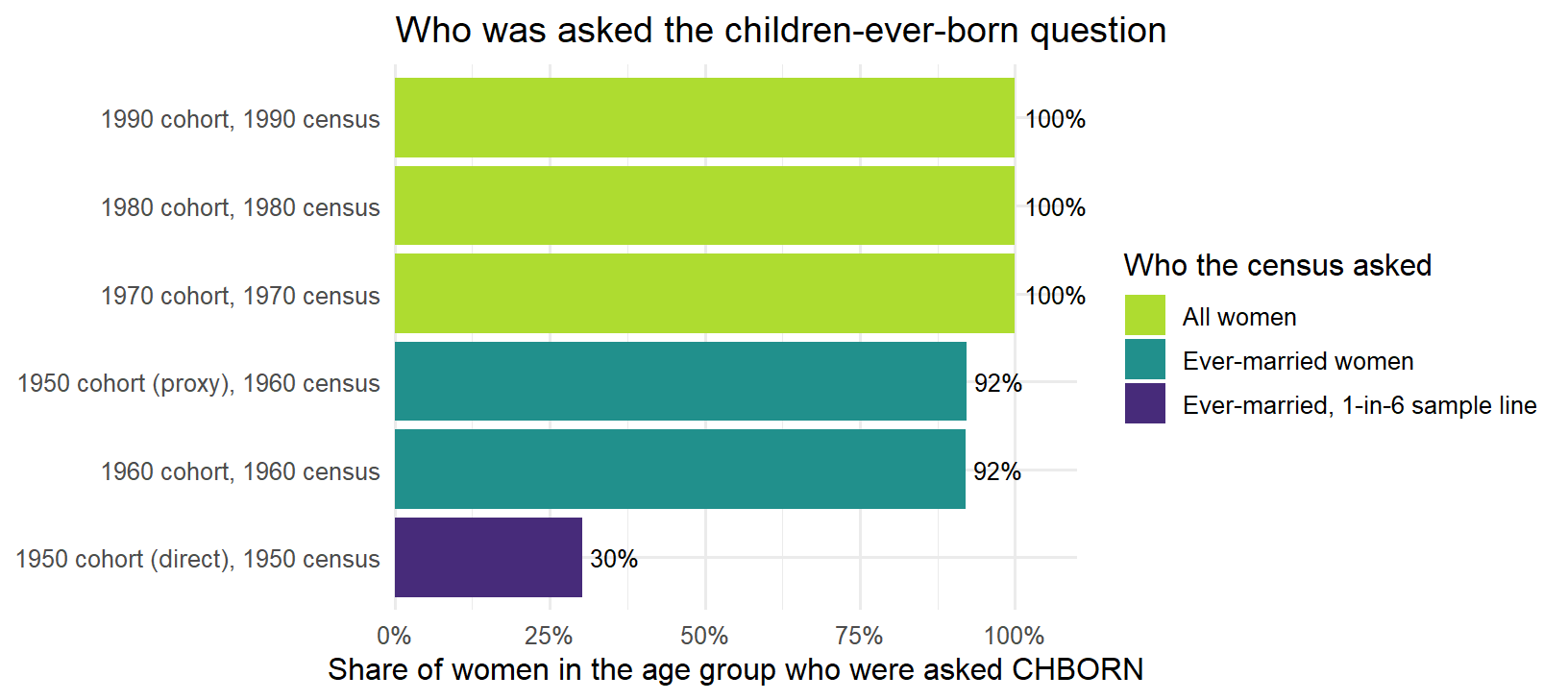
Consequence 1 — coverage (1950). Because 1950 asked only ever-married sample-line women, most 1950 women have no CHBORN value. The figure below shows, for each census/age group, the share of women who were asked the question: direct-1950 is near 30% (only ever-married sample-line women); the 1960 census — the source of both the 1960 cohort and the 1950 proxy — is near 92% (ever-married women only); and the 1970–1990 censuses are at 100% (all women). This is why the 1950 cohort is taken from a proxy (the same birth cohort observed in 1960) rather than directly (see Defining the analytic sample).

Code
coverage_labels <- tibble(
  cohort_source = c("direct_1950_validation", "proxy_1950", "main_1960",
                    "main_1970", "main_1980", "main_1990"),
  slice = c("1950 cohort (direct)", "1950 cohort (proxy)", "1960 cohort",
            "1970 cohort", "1980 cohort", "1990 cohort"),
  who_asked = c("Ever-married, 1-in-6 sample line", "Ever-married women",
                "Ever-married women", "All women", "All women", "All women")
)

chborn_universe %>%
  left_join(coverage_labels, by = "cohort_source") %>%
  mutate(label = paste0(slice, ", ", source_year, " census")) %>%
  ggplot(aes(x = reorder(label, valid_share), y = valid_share, fill = who_asked)) +
  geom_col() +
  geom_text(aes(label = scales::label_percent(accuracy = 1)(valid_share)),
            hjust = -0.15, size = 3.4) +
  coord_flip(clip = "off") +
  scale_y_continuous(labels = scales::label_percent(), limits = c(0, 1.1),
                     expand = expansion(mult = c(0, 0))) +
  scale_fill_manual(values = coverage_palette) +
  labs(x = NULL, y = "Share of women in the age group who were asked CHBORN",
       fill = "Who the census asked",
       title = "Who was asked the children-ever-born question")
Figure 1: Of the women in each census/age group, the share who were asked the children-ever-born question (i.e., were in the variable’s universe). Colour indicates whom each census asked: in 1950 only ever-married women on the 1-in-6 sample line (~30%); in 1960 only ever-married women (~92%); from 1970 all women (~100%). The low 1950 coverage is why the 1950 cohort is taken from the 1960 proxy.

Consequence 2 — the universe shift (comparability). The early cohorts describe ever-married women only; the later cohorts describe all women. A raw cross-cohort series therefore mixes two populations: the 1970–1990 samples include never-married (largely childless) women that the 1950 and 1960 samples cannot. The only universe common to every census is ever-married women, which can be reconstructed in any year from marital status (MARST); this motivates the common-universe analysis below.

4 Defining the analytic sample

The analytic population is women (SEX == 2) observed at completed fertility. Cohort membership for the main series is defined by age within a census — women aged 50–59 — not by birth year, so nobody in the age window is dropped because their birthday had not yet occurred by the April-1 census date. Birth-year spans are derived from the data afterwards, for labeling only.

Output year Source census Age window Derived birth years* Role
1950 1960 60–69 ~1890–1900 Main proxy for the 1950 cohort
1960 1960 50–59 ~1900–1910 Main series
1970 1970 50–59 ~1910–1920 Main series
1980 1980 50–59 ~1920–1930 Main series
1990 1990 50–59 ~1930–1940 Main series
1950 1950 50–59 ~1890–1900 Direct-1950 validation only

*A 10-year age window spans about 11 birth years (the April-1 birthday effect), so adjacent cohorts can share a boundary birth year. The exact span is derived from the data and shown below.

The 1950 cohort uses the 1960 proxy (the 1890–1900 birth cohort observed at ages 60–69 in 1960), because — per Consequence 1 above — direct 1950 retains only ~30% of women. Direct-1950 is computed and reported only as a validation check.

Code
age_cohort_validation %>%
  select(series, cohort_source, source_year, Year, cohort, age_min, age_max, n_records) %>%
  kable(caption = "Cohort composition: age range and derived birth-year span for each age-defined cohort slice (no records are dropped by age).")
Table 1: Cohort composition: age range and derived birth-year span for each age-defined cohort slice (no records are dropped by age).
series cohort_source source_year Year cohort age_min age_max n_records
validation direct_1950_validation 1950 1950 1891-1900 50 59 73555
main proxy_1950 1960 1950 1890-1900 60 69 70195
main main_1960 1960 1960 1900-1910 50 59 93672
main main_1970 1970 1970 1910-1920 50 59 109678
main main_1980 1980 1980 1920-1930 50 59 613086
main main_1990 1990 1990 1931-1940 50 59 587159

5 CHBORN coding and harmonization

ipumsr returns the raw IPUMS codes. Code 00 is not applicable (not in universe — not zero children); zero children is code 01, one child 02, and so on. Per the IPUMS user note, children ever born is the code minus one, after dropping 00. We keep codes 01–61, set n_child = CHBORN − 1, and cap at 12 (12+) so all cohorts share one top category: the 1960–1990 samples top-code at 12+ (code 13), while 1950 resolves higher (to 25+, code 26).

Code
value_labels %>%
  filter(var_name %in% c("SEX", "CHBORN", "MARST")) %>%
  kable(caption = "DDI value labels for the variables that drive the coding rules.")
tibble(
  raw_code = c("0", "1", "2-12", "13", "14-61", "97, 98, 99"),
  ddi_meaning = c(
    "N/A (not in universe)",
    "No children",
    "1 to 11 children",
    "12 children; 12+ in 1960-1990",
    "13 to 60 children (1950 coding)",
    "Unknown, illegible, or missing"
  ),
  harmonized_use = c(
    "Drop (not zero children)",
    "n_child = 0",
    "n_child = CHBORN - 1",
    "n_child = 12 (the 12+ bucket)",
    "n_child = 12 (the 12+ bucket)",
    "Drop"
  )
) %>%
  kable(caption = "Harmonized CHBORN coding used in all processed outputs.")
Table 2: Harmonized CHBORN coding used in all processed outputs.
var_name val lbl
SEX 1 Male
SEX 2 Female
CHBORN 0 N/A (not in universe)
CHBORN 1 No children
CHBORN 13 12 children; 12+ in 1960-1990
CHBORN 97-99 Unknown, illegible, or missing
MARST 1-5 Ever-married
MARST 6 Never-married
MARST 9 Blank/missing
raw_code ddi_meaning harmonized_use
0 N/A (not in universe) Drop (not zero children)
1 No children n_child = 0
2-12 1 to 11 children n_child = CHBORN - 1
13 12 children; 12+ in 1960-1990 n_child = 12 (the 12+ bucket)
14-61 13 to 60 children (1950 coding) n_child = 12 (the 12+ bucket)
97, 98, 99 Unknown, illegible, or missing Drop

6 Putting cohorts on a common universe

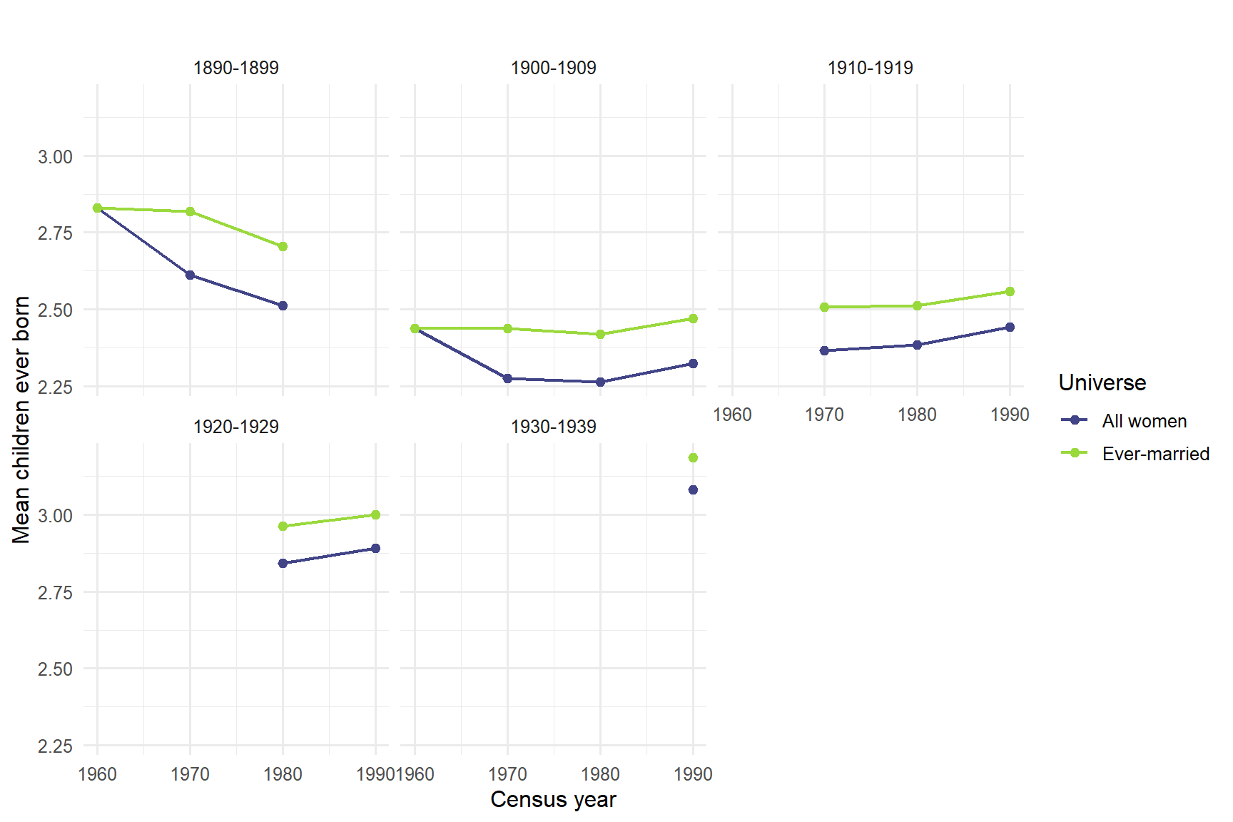
We treat fertility as effectively complete by age 50; the 50–59 age window is chosen to capture completed fertility while limiting the mortality selection that affects older ages. Under this assumption, differences in a fixed birth cohort’s measured children-ever-born distribution across successive censuses reflect measurement — mortality selection, migration, response error, and universe or top-code differences — rather than a change in fertility. We therefore estimate the universe effect by comparing the two universes within a single census, and use the cross-census comparison only to gauge the magnitude of these measurement differences.

We follow each decade birth cohort across the 1960–1990 censuses, restricting to cells where the whole cohort has reached age 50+, and within each census compute the children-ever-born distribution two ways: all women vs ever-married (MARST 1–5). Before 1970 the two coincide by construction (never-married women were not in the universe), so the contrast is informative only for 1970 onward.

Code
band_summary %>%
  mutate(Universe = recode(universe, all_women = "All women", ever_married = "Ever-married")) %>%
  ggplot(aes(universe_year, mean_children, color = Universe, group = Universe)) +
  geom_line(linewidth = 0.8) +
  geom_point(size = 2) +
  facet_wrap(~ birth_band) +
  scale_color_manual(values = universe_palette) +
  scale_x_continuous(breaks = c(1960, 1970, 1980, 1990)) +
  labs(x = "Census year", y = "Mean children ever born",
       title = "")
ggsave(file = file.path(output_path, "cohort_trajectory.pdf"), width = 9, height = 6)
Figure 2: Mean children ever born for each decade birth cohort, followed across censuses, under the two universes. The series coincide in 1960 (only ever-married women were asked) and separate from 1970 onward (all women asked); the gap between the series is the universe effect, while the drift along each line reflects mortality selection and decade differences from observing a cohort at older ages.
Code
band_pmf %>%
  filter(birth_band %in% c("1890-1899", "1900-1909"), universe_year == 1970) %>%
  mutate(Universe = recode(universe, all_women = "All women", ever_married = "Ever-married")) %>%
  ggplot(aes(n_child, probability, fill = Universe)) +
  geom_col(position = position_dodge(width = 0.8), width = 0.75) +
  facet_wrap(~ birth_band) +
  scale_fill_manual(values = universe_palette) +
  scale_x_continuous(breaks = 0:12) +
  labs(x = "Children ever born (12 = 12+)", y = "Probability",
       title = "All-women vs ever-married PMFs, early cohorts, 1970")
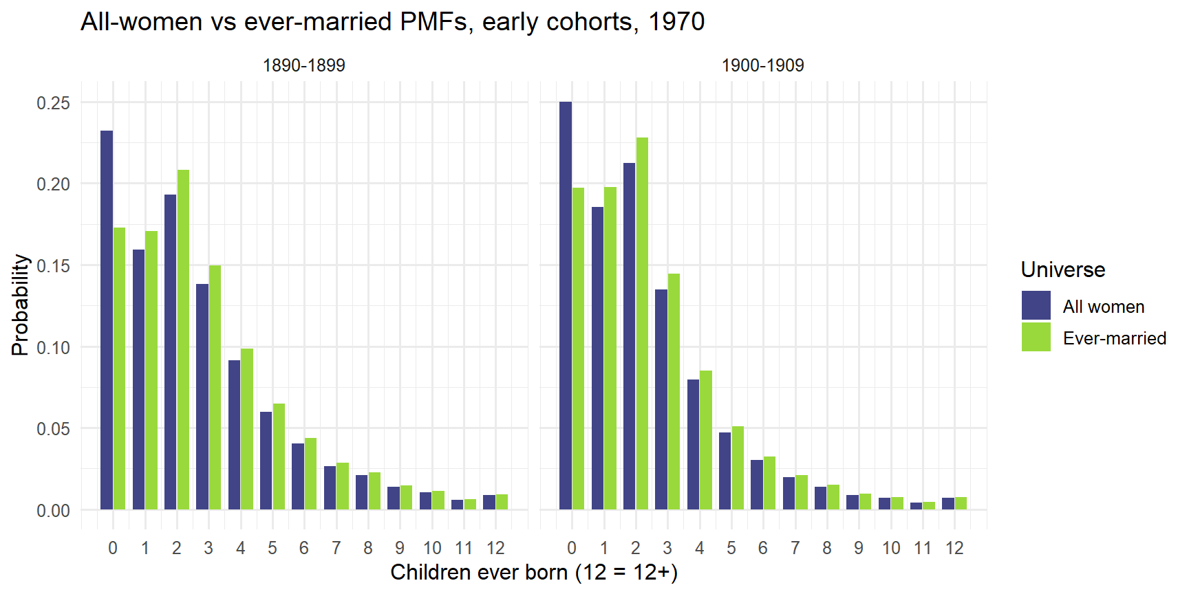
Figure 3: Children-ever-born PMFs for the two early cohorts in the first census where all women were asked (1970). Ever-married (the only universe available for these cohorts at completed fertility in 1960) vs all women. Including never-married women adds mass at zero and lowers the mean.
Code
universe_contrast %>%
  filter(universe_year >= 1970) %>%
  ggplot(aes(factor(universe_year), mean_shift, fill = birth_band)) +
  geom_col(position = position_dodge(width = 0.8), width = 0.75) +
  geom_hline(yintercept = 0, linewidth = 0.3) +
  scale_fill_manual(
    values = setNames(
      viridis(length(unique(universe_contrast$birth_band)), option = "D", begin = 0.12, end = 0.88),
      sort(unique(universe_contrast$birth_band))
    )
  ) +
  labs(x = "Census year", y = "Mean shift (all women − ever-married)",
       fill = "Birth cohort",
       title = "Effect of widening the universe to all women")
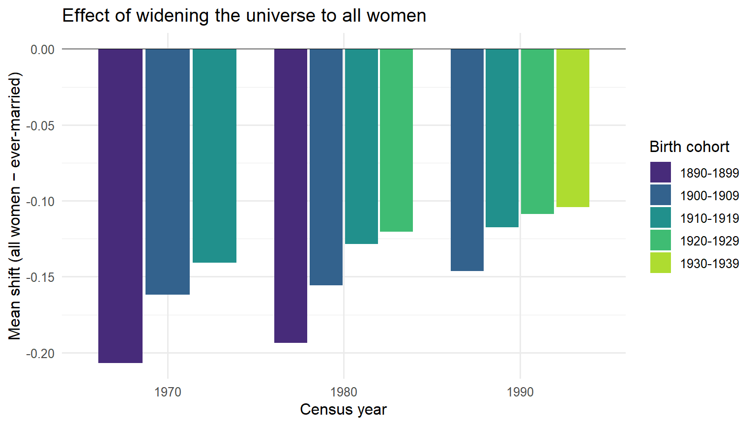
Figure 4: The universe effect: how much the mean falls when the universe is widened from ever-married to all women, by cohort and census (1970+ only, where the two universes differ).

The contrast and decomposition tables accompany the figures:

Code
universe_contrast %>%
  filter(universe_year >= 1970) %>%
  transmute(
    birth_band, universe_year,
    mean_all = mean_children_all_women,
    mean_em = mean_children_ever_married,
    mean_shift, share0_shift, pct_never_married, tvd
  ) %>%
  kable(digits = 3, caption = "All-women vs ever-married contrast by cohort and census (1970+). mean_shift = all − ever-married; pct_never_married = never-married share of the all-women cell; tvd = total-variation distance between the two PMFs.")
early_cohort_followup %>%
  kable(digits = 3, caption = "Early-cohort decomposition. universe_effect (all − ever-married in the later census) isolates the effect of adding never-married women; mortality_effect (ever-married, later − completion census) isolates survivor selection and decade artifacts.")
Table 3: Early-cohort decomposition. universe_effect (all − ever-married in the later census) isolates the effect of adding never-married women; mortality_effect (ever-married, later − completion census) isolates survivor selection and decade artifacts.
birth_band universe_year mean_all mean_em mean_shift share0_shift pct_never_married tvd
1890-1899 1970 2.612 2.819 -0.207 0.060 0.079 0.060
1890-1899 1980 2.511 2.704 -0.194 0.058 0.074 0.058
1900-1909 1970 2.276 2.438 -0.162 0.053 0.074 0.053
1900-1909 1980 2.263 2.419 -0.156 0.051 0.068 0.051
1900-1909 1990 2.324 2.470 -0.146 0.048 0.063 0.048
1910-1919 1970 2.365 2.506 -0.141 0.047 0.063 0.047
1910-1919 1980 2.383 2.511 -0.128 0.042 0.055 0.042
1910-1919 1990 2.441 2.559 -0.117 0.038 0.050 0.038
1920-1929 1980 2.843 2.964 -0.120 0.036 0.047 0.036
1920-1929 1990 2.892 3.001 -0.109 0.032 0.042 0.032
1930-1939 1990 3.082 3.186 -0.104 0.030 0.042 0.030
birth_band completed_year later_year completed_em_mean later_em_mean later_all_mean universe_effect mortality_effect
1890-1899 1960 1970 2.831 2.819 2.612 -0.207 -0.012
1900-1909 1960 1970 2.436 2.438 2.276 -0.162 0.001

Interpretation. The within-census all-women vs ever-married contrast (mean_shift, tvd, and the 1970 PMFs) is the preferred estimate: it compares the same survivors in the same census, with appropriate PERWT weighting. Differences across censuses — the drift along each trajectory — bound the combined measurement difference rather than a change in fertility. Key caveats:

  • Mortality selection. Never-married women have higher old-age mortality, so the all-women pool drifts toward ever-married at older ages — the universe gap is attenuated at older ages. The least-contaminated estimate is the contrast at the youngest census in which a cohort is observed under the all-women universe.
  • Never-married fertility is a lower bound. Historically nonmarital births are under-reported, so the all-women mean understates true all-women fertility and the gap is, if anything, overstated.
  • Weighting. PERWT is appropriate for 1970–1990 (CHBORN is universal there), so the within-census contrast is unaffected by the weighting issue below. 1950 is excluded from this analysis (its sample-line weight SLWT is absent), and the 1960 cells are ever-married by construction.
  • Migration / nativity. Birth cohorts are not closed across censuses; NATIVITY/BPL are absent, so cross-census comparisons cannot be restricted to the native-born — a further reason to rely on the within-census contrast, which compares a single population. gq_household_share is reported per cell as a coarse check on institutionalization at older ages.

In sum, the pre-1970 cohorts (1950 and 1960) are observed only for ever-married women, which raises their measured completed fertility by roughly 0.1–0.2 children relative to an all-women basis. This gap is small next to the Depression-era decline in completed fertility across the 1901–1920 birth cohorts, and it is reported as a sensitivity rather than applied to the main series.

7 Aggregate fertility distributions

The main-series outputs — completed-fertility distributions for women 50–59, with the 1950 proxy — are the inputs read by the downstream model and simulator. Means are reported unweighted, the form those downstream steps require; PERWT-weighted versions are written alongside as a sensitivity.

Code
cohort_means %>%
  filter(series == "main") %>%
  ggplot(aes(Year, mean_children)) +
  geom_line(linewidth = 0.8, color = main_series_color) +
  geom_point(size = 2.5, color = main_series_color) +
  geom_text(aes(label = round(mean_children, 2)), vjust = -0.9, size = 3.3) +
  scale_x_continuous(breaks = c(1950, 1960, 1970, 1980, 1990)) +
  labs(x = "Cohort (census year)", y = "Mean children ever born",
       title = "Completed fertility by cohort")
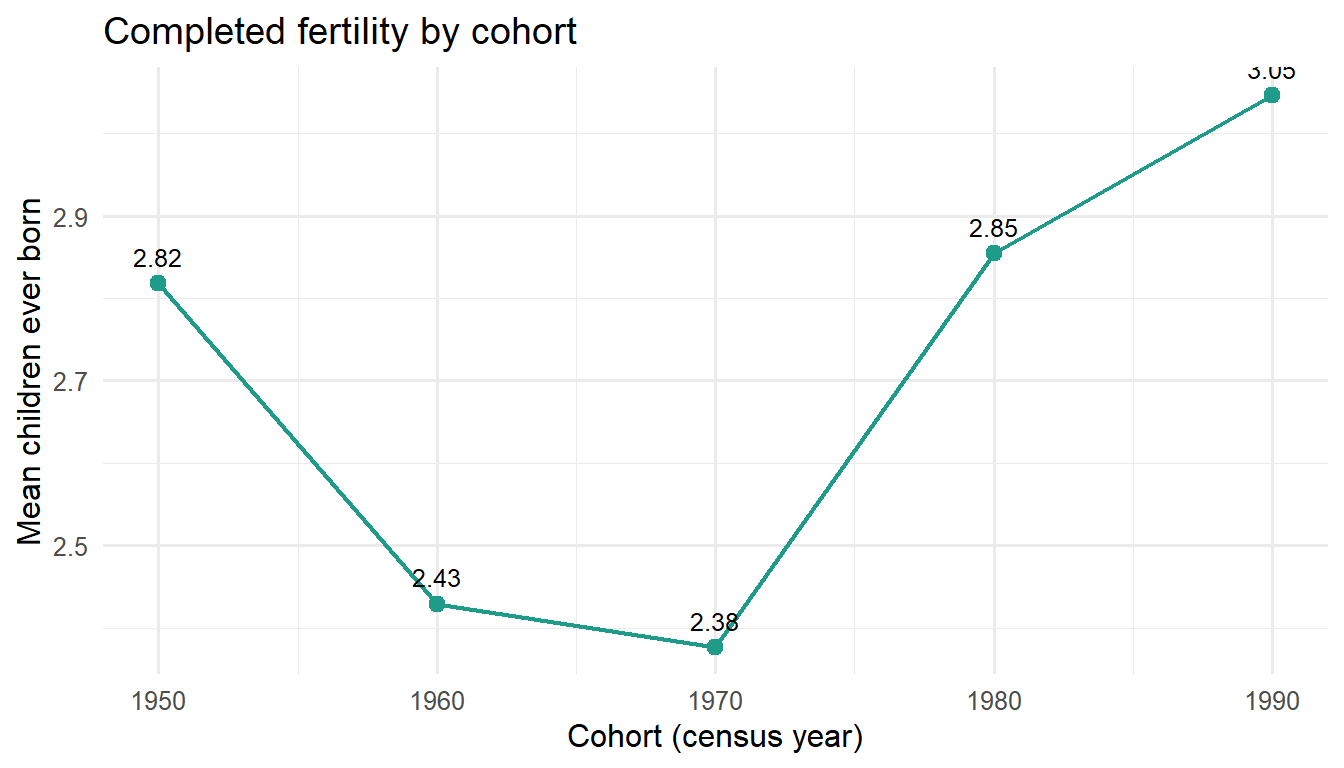
Figure 5: Mean children ever born by main-series cohort (women 50-59; 1950 is the 1960 proxy). The dip for the 1901-1920 cohorts and the rise for the baby-boom mothers are demographically expected.
Code
fertility_pmf %>%
  ggplot(aes(children, probability)) +
  geom_col(fill = main_series_color, width = 0.8) +
  facet_wrap(~ Year) +
  scale_x_continuous(breaks = 0:12) +
  labs(x = "Children ever born (12 = 12+)", y = "Probability",
       title = "Fertility PMFs by cohort")
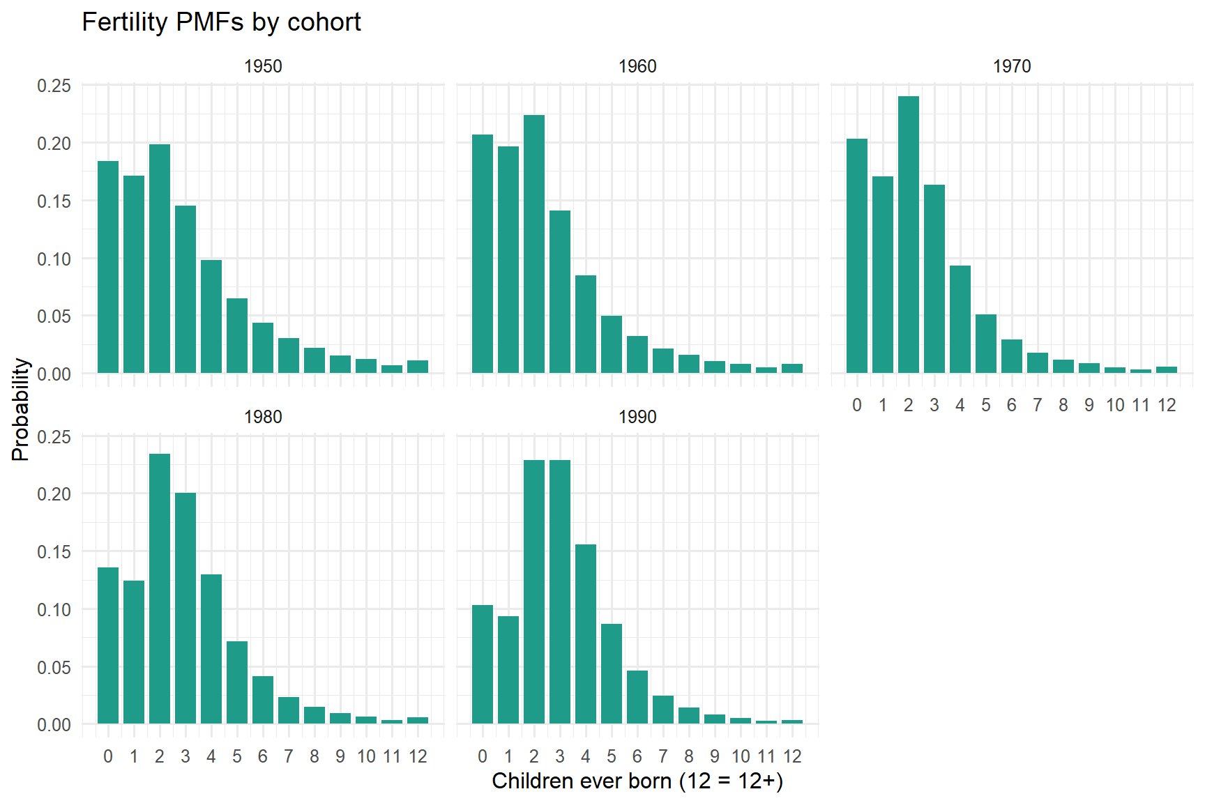
Figure 6: Fertility distributions (children ever born, 12 = 12+) for each main-series cohort.
Code
cohort_sample_sizes %>%
  kable(digits = 0, caption = "Main-series cohort sample sizes (unweighted and PERWT-weighted).")
cohort_means %>%
  filter(series == "main") %>%
  transmute(Year, cohort, n_women, mean_children, mean_children_weighted, share_12plus) %>%
  kable(digits = 3, caption = "Main-series mean children ever born and 12+ shares (unweighted and weighted).")
Table 4: Main-series mean children ever born and 12+ shares (unweighted and weighted).
Year cohort n_women n_women_weighted
1950 1890-1900 64760 6451460
1960 1900-1910 86233 8590203
1970 1910-1920 109678 10967800
1980 1920-1930 613086 12261720
1990 1931-1940 587159 11360431
Year cohort n_women mean_children mean_children_weighted share_12plus
1950 1890-1900 64760 2.818 2.818 0.011
1960 1900-1910 86233 2.429 2.429 0.008
1970 1910-1920 109678 2.377 2.377 0.006
1980 1920-1930 613086 2.855 2.855 0.006
1990 1931-1940 587159 3.047 3.003 0.003

8 Validation: direct vs proxy 1950

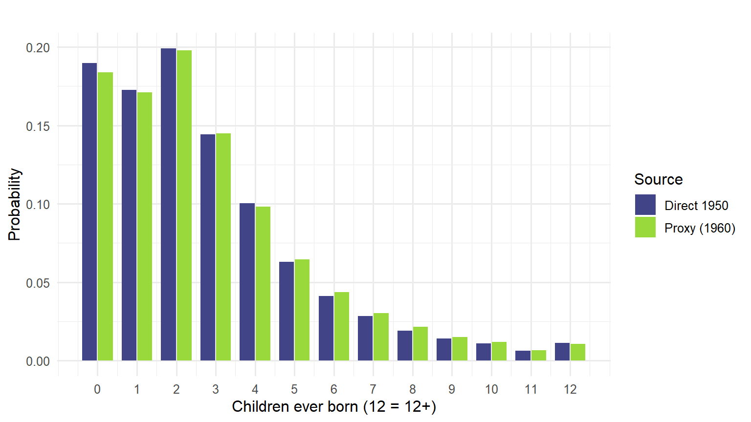
The 1950 cohort is represented by the 1960 proxy. As a check, we compare it against the held-out direct-1950 records (women 50–59 in the 1950 census). The unweighted distributions are nearly identical, which corroborates the proxy. (The weighted direct-1950 number is unreliable — 1950 CHBORN is a sample-line variable and the correct weight SLWT is not in the extract — so we rely on the unweighted comparison, and tail differences above 12 are affected by the top-code asymmetry noted in the coding section.)

Code
validation_1950_pmf %>%
  mutate(Source = recode(cohort_source,
                         direct_1950_validation = "Direct 1950",
                         proxy_1950 = "Proxy (1960)")) %>%
  ggplot(aes(n_child, probability, fill = Source)) +
  geom_col(position = position_dodge(width = 0.8), width = 0.75) +
  scale_fill_manual(values = validation_palette) +
  scale_x_continuous(breaks = 0:12) +
  labs(x = "Children ever born (12 = 12+)", y = "Probability",
       title = "")
ggsave(file = file.path(output_path, "validation_1950_pmf.pdf"), width = 8, height = 4.5)
Figure 7: Children-ever-born PMFs (unweighted): direct 1950 (women 50-59 in 1950) vs the 1960 proxy (women 60-69 in 1960). Near-identical shapes corroborate using the proxy.
Code
validation_1950_summary %>%
  kable(digits = 3, caption = "Direct 1950 vs proxy 1950 summary. Unweighted means agree closely; the weighted direct-1950 number is approximate (no SLWT).")
Table 5: Direct 1950 vs proxy 1950 summary. Unweighted means agree closely; the weighted direct-1950 number is approximate (no SLWT).
cohort_source source_year output_year n_women n_women_weighted mean_children mean_children_weighted share_12plus
direct_1950_validation 1950 1950 22263 3010813 2.758 2.330 0.011
proxy_1950 1960 1950 64760 6451460 2.818 2.818 0.011

9 Limitations

  • 12+ top-code. All outputs harmonize the child-count support to 0, 1, …, 11, 12+. 1960–1990 already top-code at 12+, but 1950 resolves to 25+, so the cap discards tail detail for the (validation-only) 1950 series and for older cohorts seen in 1950.
  • Weighting. Main outputs are unweighted; PERWT-weighted versions are provided as a sensitivity. The 1950 sample-line weight SLWT is absent, so any 1950 weighted figure is approximate; 1950 is therefore kept out of the weighted cross-cohort series.
  • Extract gaps. A future extract should add SLWT (correct 1950 weighting), NATIVITY/BPL (restrict to native-born / measure cohort compositional drift across censuses), and QCHBORN (filter allocated/imputed values). Each would close a caveat that the current data cannot resolve.
  • Sharing. The restricted IPUMS records, person-level weights, and raw fixed-width data remain local-only and are not committed; only the aggregate CSVs are.

10 Appendix: reproducibility and outputs

This page is processed-data-first: a normal render loads the committed aggregate CSVs from data/processed/ and does not look for or open restricted raw IPUMS files. Set KINCOUNTS_REBUILD_IPUMS=true to explicitly rebuild the aggregates from a local raw extract.

Code
kable(file_summary, caption = "Local restricted IPUMS files and cache state for this render.")
kable(ddi_variables, caption = "Parsed variables and their fixed-width positions in the DDI.")
kable(
  tibble(rebuild_from_raw = rebuild_processed, processed_file_count = length(processed_files)),
  caption = "Preprocessing cache status for this render."
)
kable(written_files, caption = "Aggregate processed files available in data/processed.")
kable(output_inventory, caption = "Full inventory of aggregate output files.")
Table 6: Full inventory of aggregate output files.
item value
compressed_data_file NA
ddi_codebook NA
compressed_size_mib NA
raw_extract_used FALSE
processed_outputs_current TRUE
rebuild_from_raw FALSE
var_name var_label start end imp_decim
YEAR Raw DDI unavailable in processed-only render NA NA NA
PERWT Raw DDI unavailable in processed-only render NA NA NA
SEX Raw DDI unavailable in processed-only render NA NA NA
AGE Raw DDI unavailable in processed-only render NA NA NA
BIRTHYR Raw DDI unavailable in processed-only render NA NA NA
MARST Raw DDI unavailable in processed-only render NA NA NA
GQ Raw DDI unavailable in processed-only render NA NA NA
CHBORN Raw DDI unavailable in processed-only render NA NA NA
rebuild_from_raw processed_file_count
FALSE 20
file status
ipums_preprocess_metadata.csv available
ipums_cohort_sample_sizes.csv available
ipums_fertility_counts_by_cohort.csv available
ipums_fertility_pmf_by_cohort.csv available
ipums_fertility_counts_by_cohort_weighted.csv available
ipums_fertility_pmf_by_cohort_weighted.csv available
validation_1950_direct_vs_proxy.csv available
validation_1950_direct_vs_proxy_pmf.csv available
ipums_age_cohort_validation.csv available
ipums_chborn_universe_by_cohort.csv available
ipums_cohort_fertility_checks.csv available
ipums_cohort_universe_summary.csv available
ipums_cohort_universe_pmf.csv available
ipums_universe_contrast_by_cohort.csv available
ipums_early_cohort_followup.csv available
fertility_pmf_1950.csv available
fertility_pmf_1960.csv available
fertility_pmf_1970.csv available
fertility_pmf_1980.csv available
fertility_pmf_1990.csv available
file contents role
ipums_preprocess_metadata.csv Processing version and rebuild timestamp. Reproducibility check
ipums_cohort_sample_sizes.csv Main-series sample sizes by output cohort. Downstream model input
ipums_fertility_counts_by_cohort.csv Unweighted main-series fertility counts by cohort and child-count bucket. Downstream model input
ipums_fertility_pmf_by_cohort.csv Unweighted main-series fertility PMF by cohort and child-count bucket. Downstream model input
ipums_fertility_counts_by_cohort_weighted.csv PERWT-weighted main-series fertility counts. Sensitivity output
ipums_fertility_pmf_by_cohort_weighted.csv PERWT-weighted main-series fertility PMF. Sensitivity output
validation_1950_direct_vs_proxy.csv Aggregate comparison of proxy 1950 and direct 1950 validation records. Validation output
validation_1950_direct_vs_proxy_pmf.csv Child-count PMFs for proxy 1950 and direct 1950 validation records. Validation output
ipums_age_cohort_validation.csv Age range and derived birth-year span for each age-defined cohort source. QA output
ipums_chborn_universe_by_cohort.csv Valid versus not-in-universe CHBORN counts by cohort source. QA output
ipums_cohort_fertility_checks.csv Aggregate mean children and 12+ share by cohort source. QA output
ipums_cohort_universe_summary.csv Common-universe analysis: per decade-cohort x census x universe summary. Common-universe analysis
ipums_cohort_universe_pmf.csv Common-universe analysis: child-count PMFs per decade-cohort x census x universe. Common-universe analysis
ipums_universe_contrast_by_cohort.csv All-women vs ever-married contrast (mean shift, share-0 shift, TVD) by cohort. Common-universe analysis
ipums_early_cohort_followup.csv Early-cohort decomposition of universe vs mortality/decade effects. Common-universe analysis
fertility_pmf_1950.csv One unweighted main-series fertility PMF for the named output year. Downstream simulator input
fertility_pmf_1960.csv One unweighted main-series fertility PMF for the named output year. Downstream simulator input
fertility_pmf_1970.csv One unweighted main-series fertility PMF for the named output year. Downstream simulator input
fertility_pmf_1980.csv One unweighted main-series fertility PMF for the named output year. Downstream simulator input
fertility_pmf_1990.csv One unweighted main-series fertility PMF for the named output year. Downstream simulator input