Bayesian Varying Coefficient Model (BVCM) for Skin Reflectance Spectra
We implement a Bayesian Varying Coefficient Model (BVCM) to analyze and generate realistic human skin reflectance spectra based on the ISSA dataset.
Key Features:
- Models skin reflectance as a function of melanin index and erythema index
- Uses Gaussian Processes for smooth, wavelength-dependent coefficient functions
- Captures subject-specific variations through random effect GPs
- Enables synthetic spectra generation with biologically plausible characteristics
- Provides a two-stage validation filter for quality control of simra Validation Filter
1 Model specification
1.1 Mathematical formulation
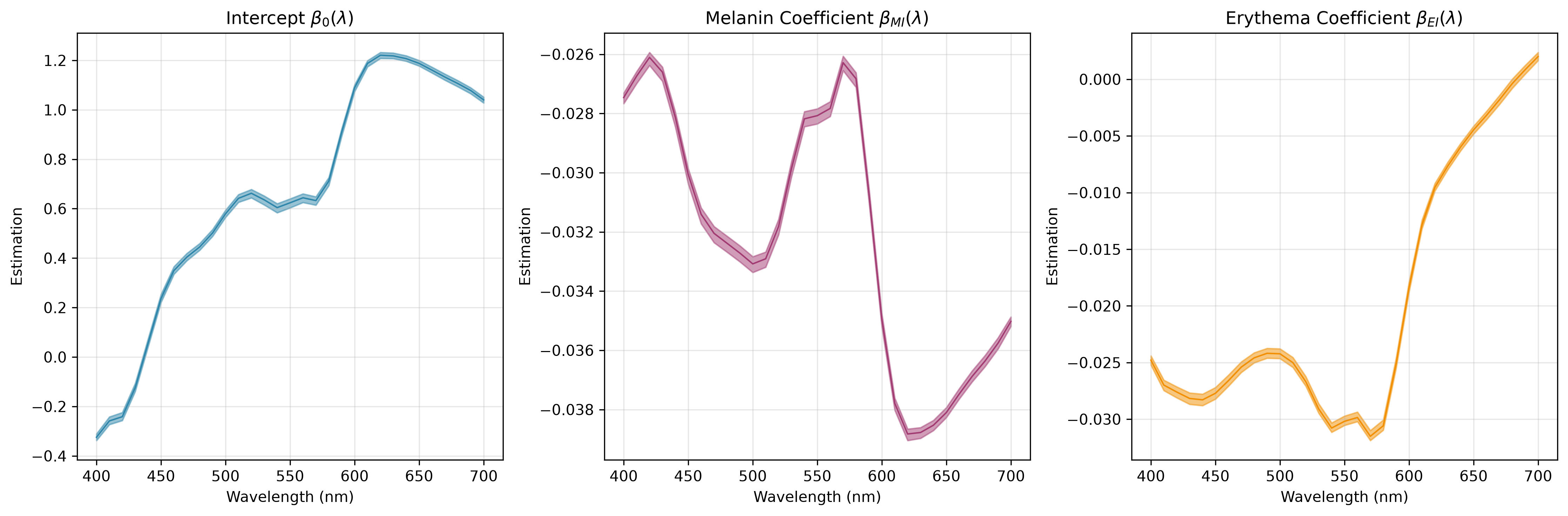
Assume we have skin reflectance spectra \(Y_i(\lambda) \in [0,1]\) for individuals \(i = 1, \ldots, N\) measured at wavelengths \(\lambda \in [400, 700]\) nm. We apply a logit transformation on the skin reflectance to ensure the transformed values are in the range \((-\infty, \infty)\). The BVCM can be formulated as: \[logit(Y_i(\lambda)) = \beta_0(\lambda) + X_{MI,i} \beta_{MI}(\lambda) + X_{EI,i} \beta_{EI}(\lambda) + Z_i(\lambda) + \epsilon_i(\lambda),\] where \(\beta_0(\lambda)\) is the intercept function, \(\beta_{MI}(\lambda)\) and \(\beta_{EI}(\lambda)\) are the varying coefficient functions for melanin and erythema variables, respectively. \(Z_i(\lambda)\) represents subject-specific deviations modeled as a Gaussian process, and \(\epsilon_i(\lambda)\) is the measurement error.
The melanin and hemoglobin variables are calculated as:
- Melanin index: \[X_{MI,i} = 100 \times \log_{10}\left(\frac{1}{R_{680,i}}\right),\] where \(R_{680,i}\) is reflectance at 680nm for individual \(i\).
- Erythema index: \[X_{EI,i} = 100 \times \log_{10}\left(\frac{R_{680,i}}{R_{560,i}}\right).\]
1.2 Spline basis representation and Hilbert space GP priors
We represent the intercept and coefficient functions using cubic P-spline basis functions. Each function is expressed as: \[\beta_k(\lambda) = \sum_{j=1}^{J} b_{k,j} B_j(\lambda),\] where \(B_j(\lambda)\) are the spline basis functions and \(b_{k,j}\) are the coefficients. Here we set \(J=20\).
We employ the Hilbert Space Gaussian Process (HSGP) approximation to model the random effect functions \(Z_i(\lambda)\), allowing efficient computation while capturing smooth variations. We approximate the GP \(Z(\lambda)\) using a finite set of basis functions derived from the eigenfunctions of the covariance kernel: \[Z(\lambda) \approx \sum_{m=1}^{M} w_m \phi_m(\lambda),\] where \(\phi_m(\lambda)\) are the basis functions and \(w_m\) are the weights drawn from a Gaussian distribution. For a stationary kernel (like Matern) in 1D, the basis functions are sine waves determined by the domain size, and the variance of the weights is determined by the Spectral Density of the kernel. Specifically, \[Z(\lambda) \approx \sum_{m=1}^M \frac{1}{\sqrt{L}} \sin \left(\frac{m\pi(\lambda+L)}{2L}\right) \cdot \sqrt{S(\omega_m)} \cdot w_m,\] where \(L\) is half the domain length, \(S(\omega_m)\) is the spectral density at frequency \(\omega_m = \frac{m\pi}{2L}\), and \(w_m \sim \mathcal{N}(0,1)\). Here we set \(M=10\).
1.3 Prior specifications
We define the following prior distributions for the model parameters:
- Random walk priors for spline coefficients:
- \[\Delta^2 b_{k,j} = b_{k,j} - 2b_{k,j-1} + b_{k,j-2} \sim N(0, \tau_{\beta}^2),\] where \(\tau_{\beta}=1\) controls the smoothness of the coefficient functions.
- Gaussian Process prior for subject-specific deviations:
- \[Z_i(\lambda) \sim GP(0, K_{Z}(\lambda, \lambda')),\] where \(K_{Z}(\lambda, \lambda')\) is a Matern52 covariance function with length \(\rho_{Z}\) and scale \(\sigma_{Z}\).
- \[\rho_{Z} \sim Gamma(50, 1), \quad \sigma_{Z} \sim HalfNormal(0.5).\]
- Normal prior for measurement error:
- \[\epsilon_i(\lambda) \sim N(0, \sigma_{\epsilon}^2),\] where \(\sigma_{\epsilon}^2\) is the variance of the measurement error.
- \[\sigma_{\epsilon}^2 \sim IG(1, 1).\]
2 Exploratory analysis on ISSA face sites
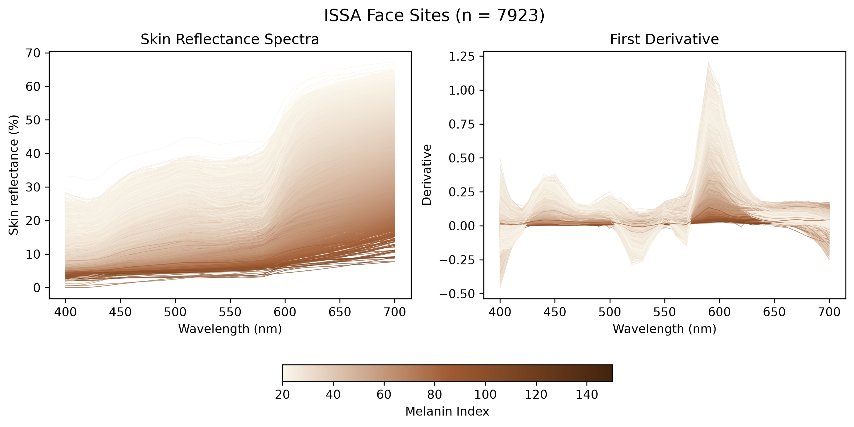
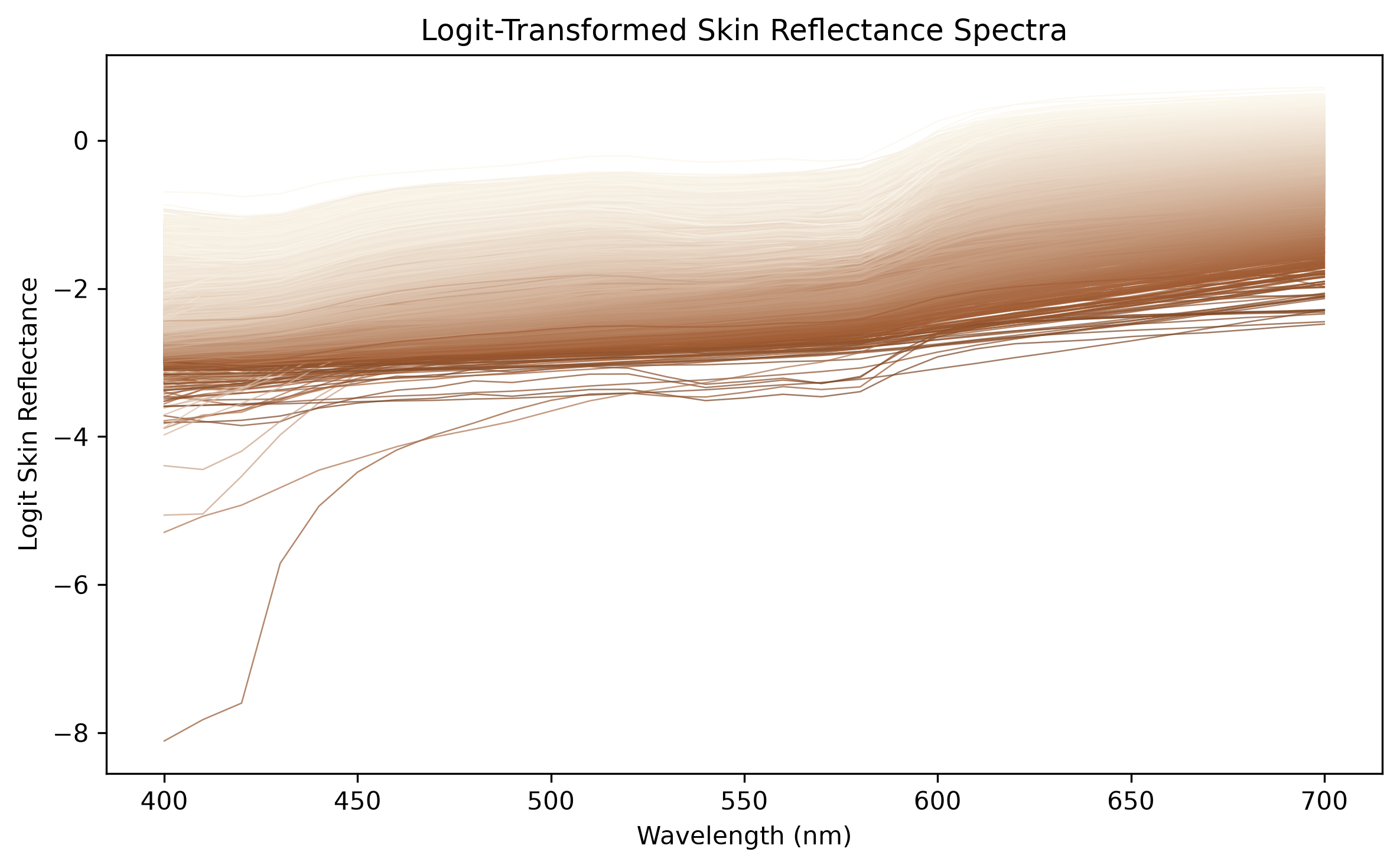
2.1 Skin reflectance and its first derivative
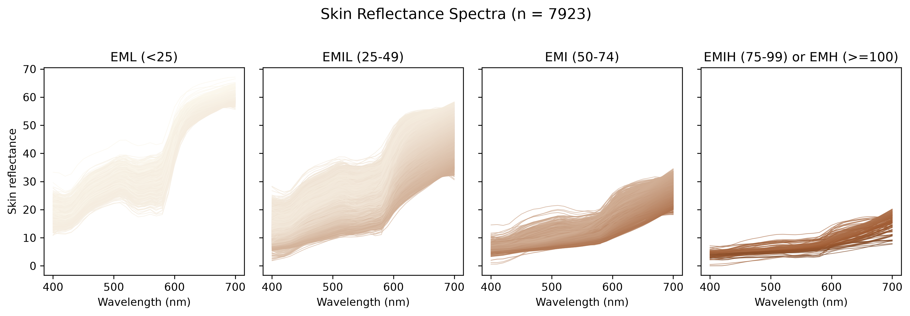
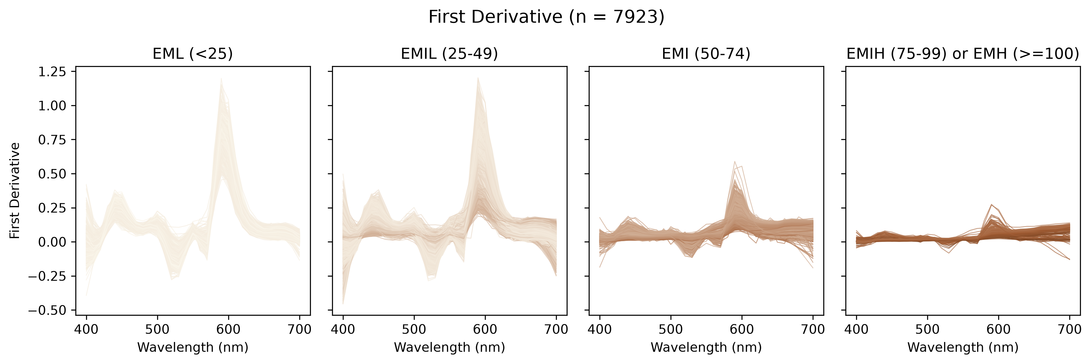
2.2 Eumelanin human skin colour scale
ISSA Face Sites Eumelanin Class Summary Table:
| Eumelanin Class | EML (<25) | EMIL (25-49) | EMI (50-74) | EMIH (75-99) | EMH (>=100) |
|---|---|---|---|---|---|
| Site | |||||
| Cheek | 216 | 1978 | 227 | 50 | 4 |
| Cheek Bone | 24 | 186 | 18 | 0 | 0 |
| Chin | 271 | 1507 | 211 | 36 | 5 |
| Ear lobe | 9 | 394 | 57 | 12 | 3 |
| Forehead | 77 | 1772 | 190 | 30 | 3 |
| Nose tip | 29 | 582 | 31 | 1 | 0 |
| Total | 626 | 6419 | 734 | 129 | 15 |
2.3 Chromophore distribution modeling
The relationship between melanin index and erythema index is shown as:
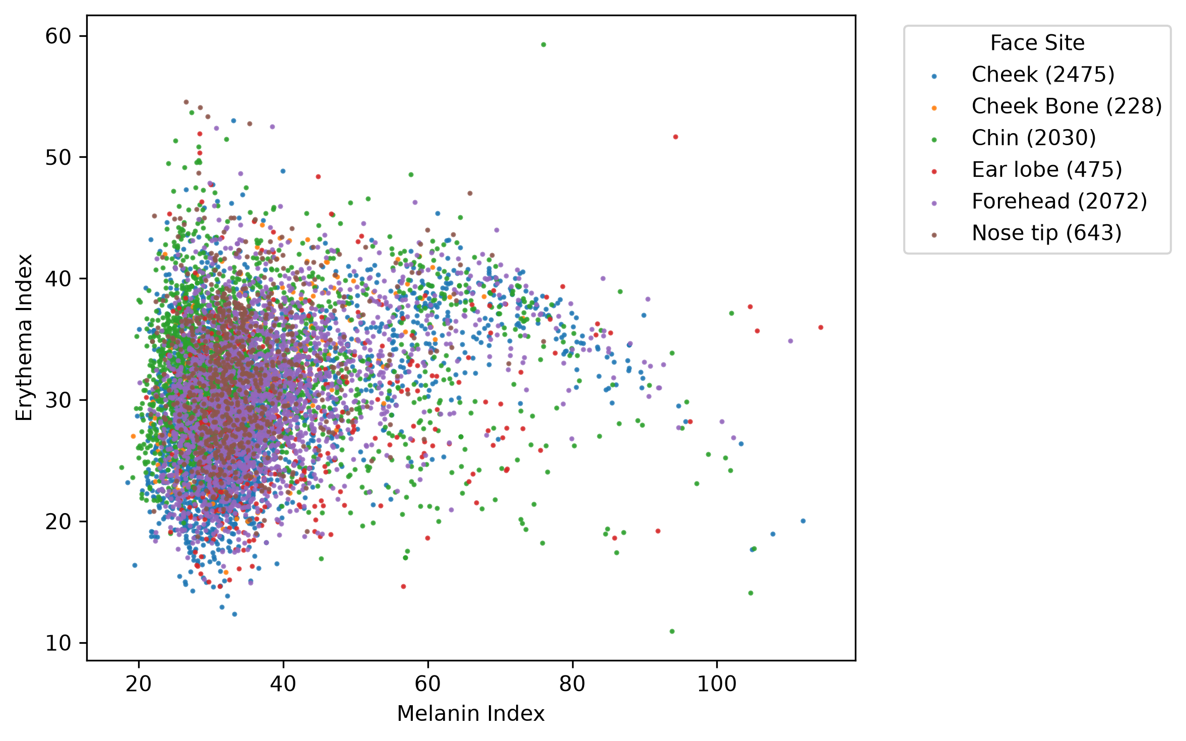
We apply a Gaussian mixture model with 5 components to approximate the distribution of melanin and erythema indices in the population. This allows us to identify the realistic combinations of these chromophore indices. The EM fit has several nearly equivalent optima, so the fitted mixture is saved to output/corrected_validation/gmm_mi_ei_reference.npz and reused, which keeps Stage 1 fixed across runs.
For Stage 1, each spectrum is assigned to its most probable component. The acceptance region of component \(k\) is the Mahalanobis ellipse whose radius is the 99th percentile of the distances of the ISSA spectra assigned to \(k\).
Loaded saved GMM: gmm_mi_ei_reference.npz
Stage 1 thresholds by component: [2.656 2.783 3.552 2.66  2.941]
ISSA facial spectra inside at least one region: 99.4%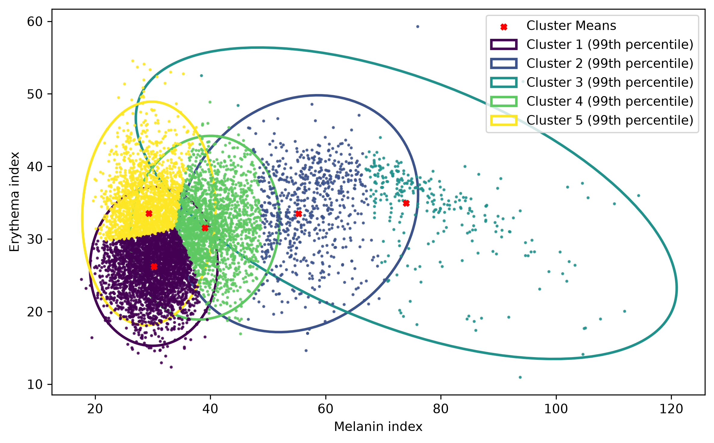
3 Posterior inference
We use the existing hybrid Gibbs model fitted to the ISSA facial spectra, with 10,000 tuning iterations and 10,000 subsequent iterations, retaining every tenth draw. A compatible checkpoint is reused when available. The downloaded bvcm_issa_face_posterior.npz contains 8,033 subject deviations and no labeled residual-covariance state, so it cannot supply the current model’s Stage 2 reference. The first run below fits the model on the current 6,338 training spectra and saves a complete compatible checkpoint.
To reduce memory use, the mean subject-specific deviation is accumulated across the same retained draws. Coefficient and hyperparameter draws remain available for posterior summaries.
3.1 Preprocess data
3.2 Gibbs sampler
Loaded compatible Gibbs checkpoint: bvcm_gibbs_validation_checkpoint.npz
Posterior means: length scale=45.844508, amplitude=0.106108, noise variance=0.00022890
3.3 Posterior visualization
3.3.1 Coefficient function estimation
3.3.2 Predict reflectance spectra given MI and EI
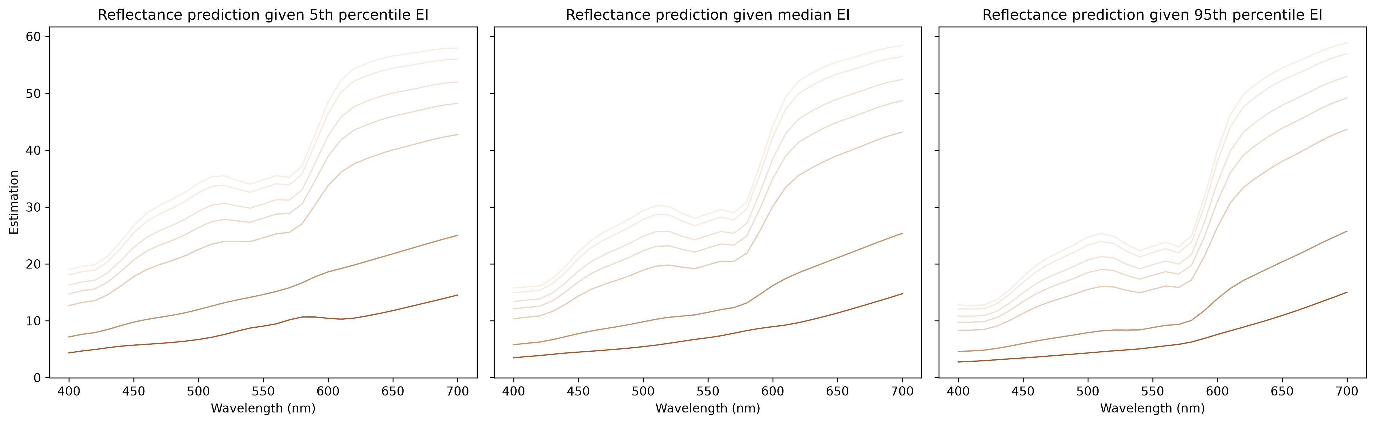
Remark: Across various levels of the erythema index, the predicted reflectance spectra exhibit a W-shape at low melanin indices and an increasing shape at high melanin indices. This finding is consistent with the shape analysis within ISSA.
3.3.3 Subject-specific deviation
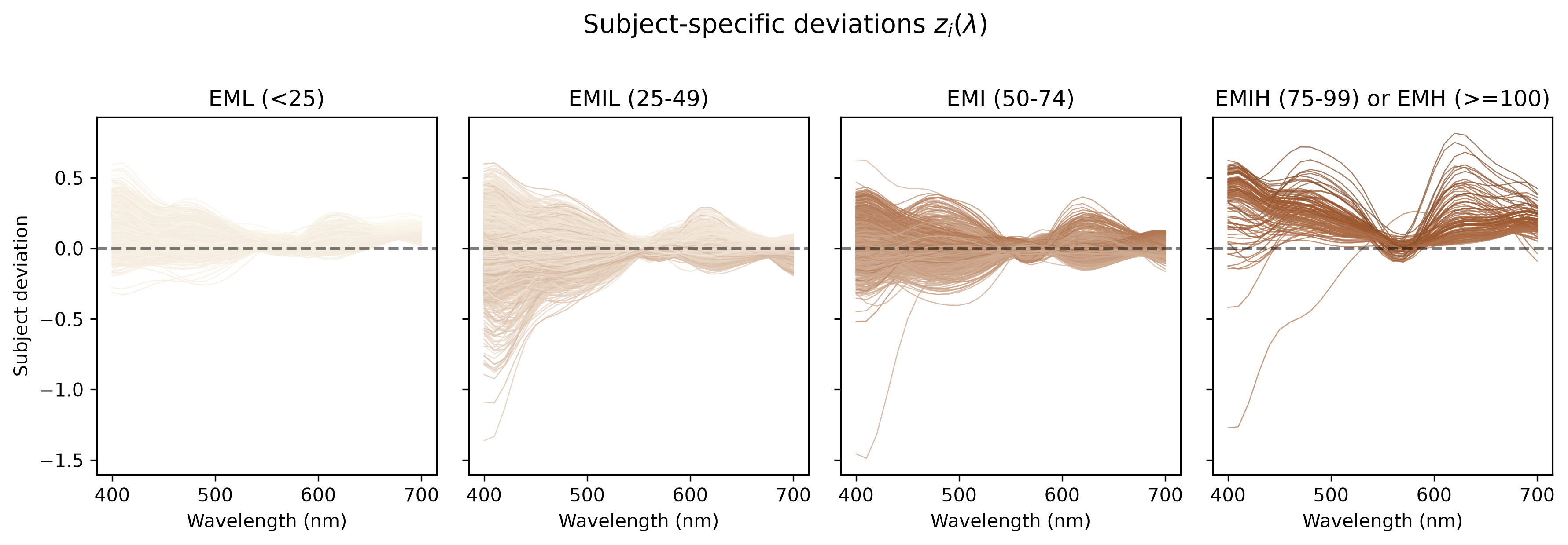
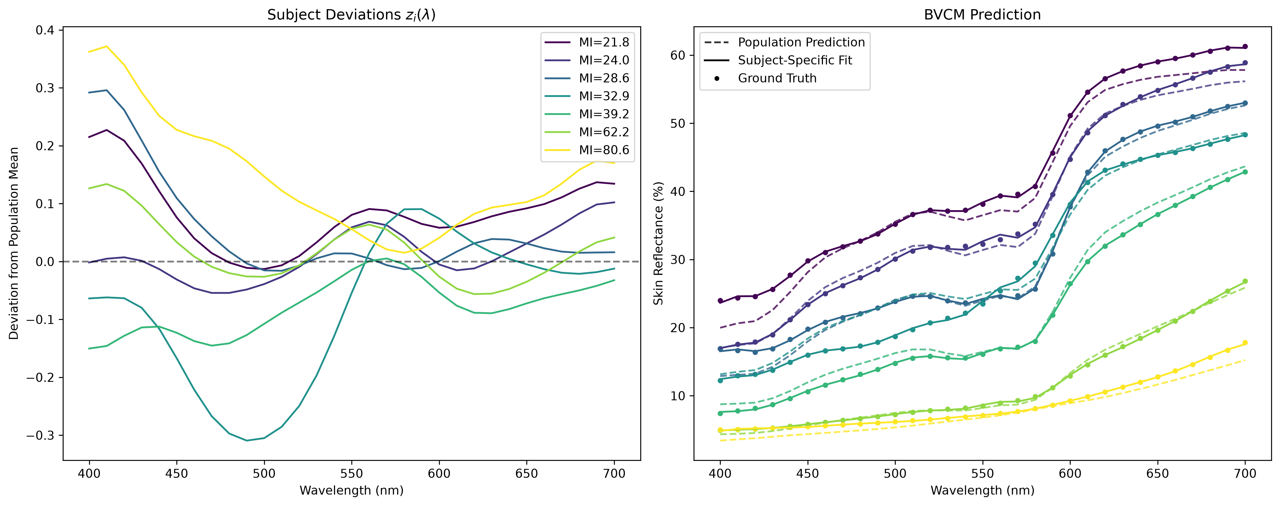
4 Model diagnostics and evaluation
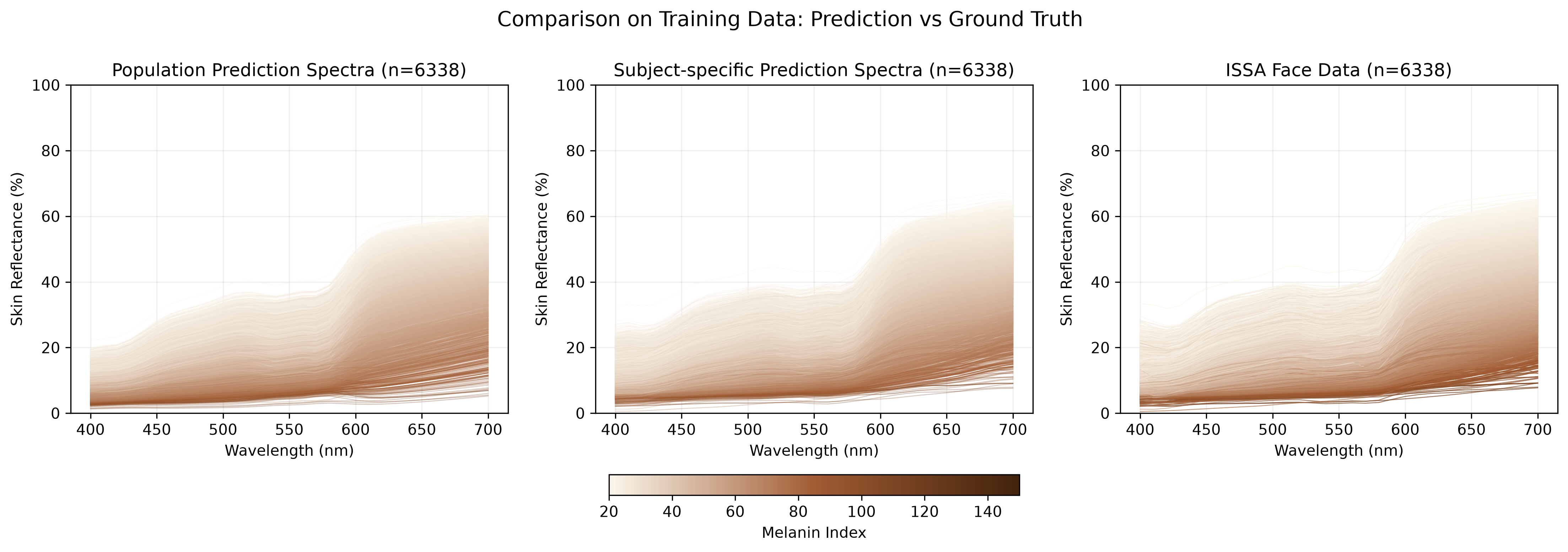
4.1 Evaluation on training data
| Model | R² | RMSE (%) | MAE (%) | |
|---|---|---|---|---|
| 0 | Population-Level (Fixed Effects) | 0.965248 | 1.411095 | 1.053455 |
| 1 | Subject-Specific (Fixed + Random) | 0.999319 | 0.197515 | 0.131818 |
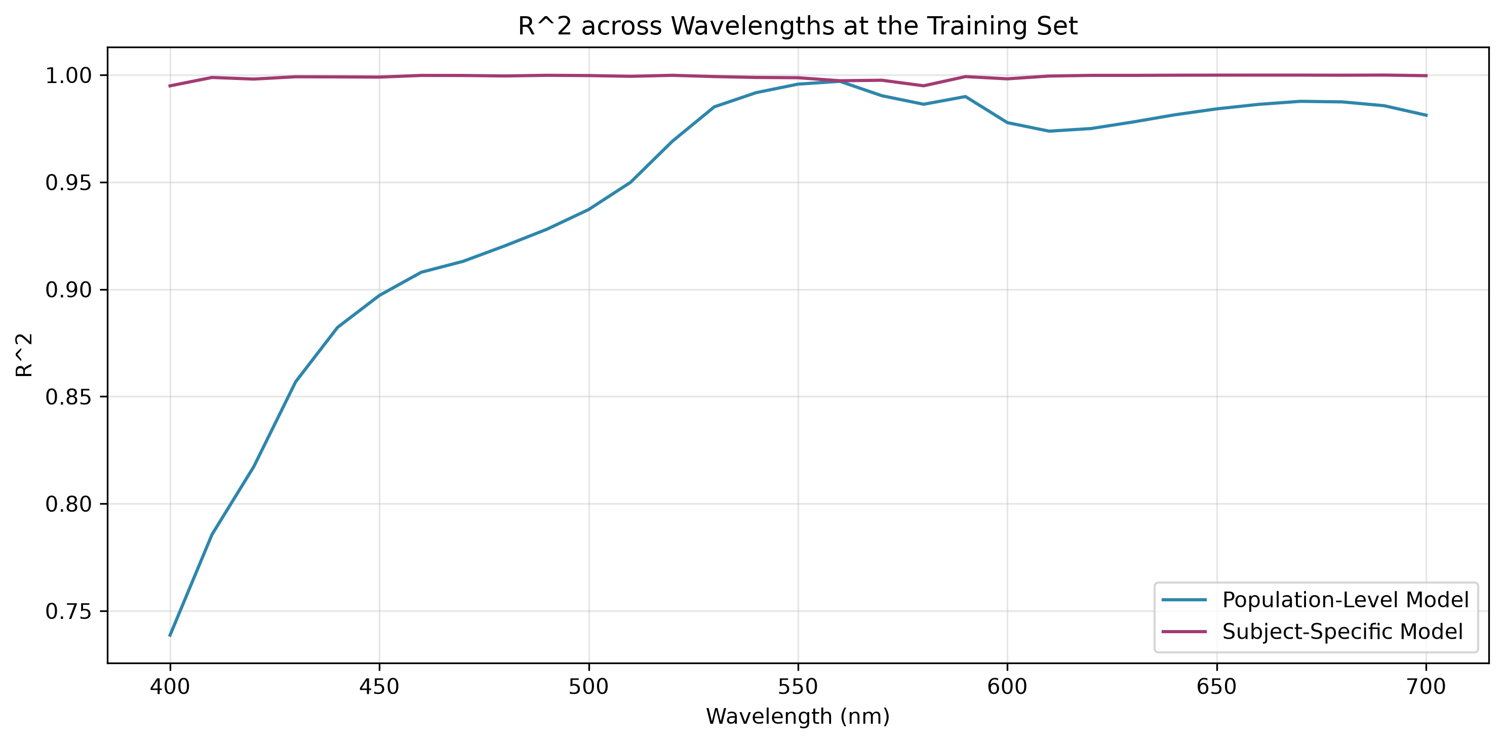
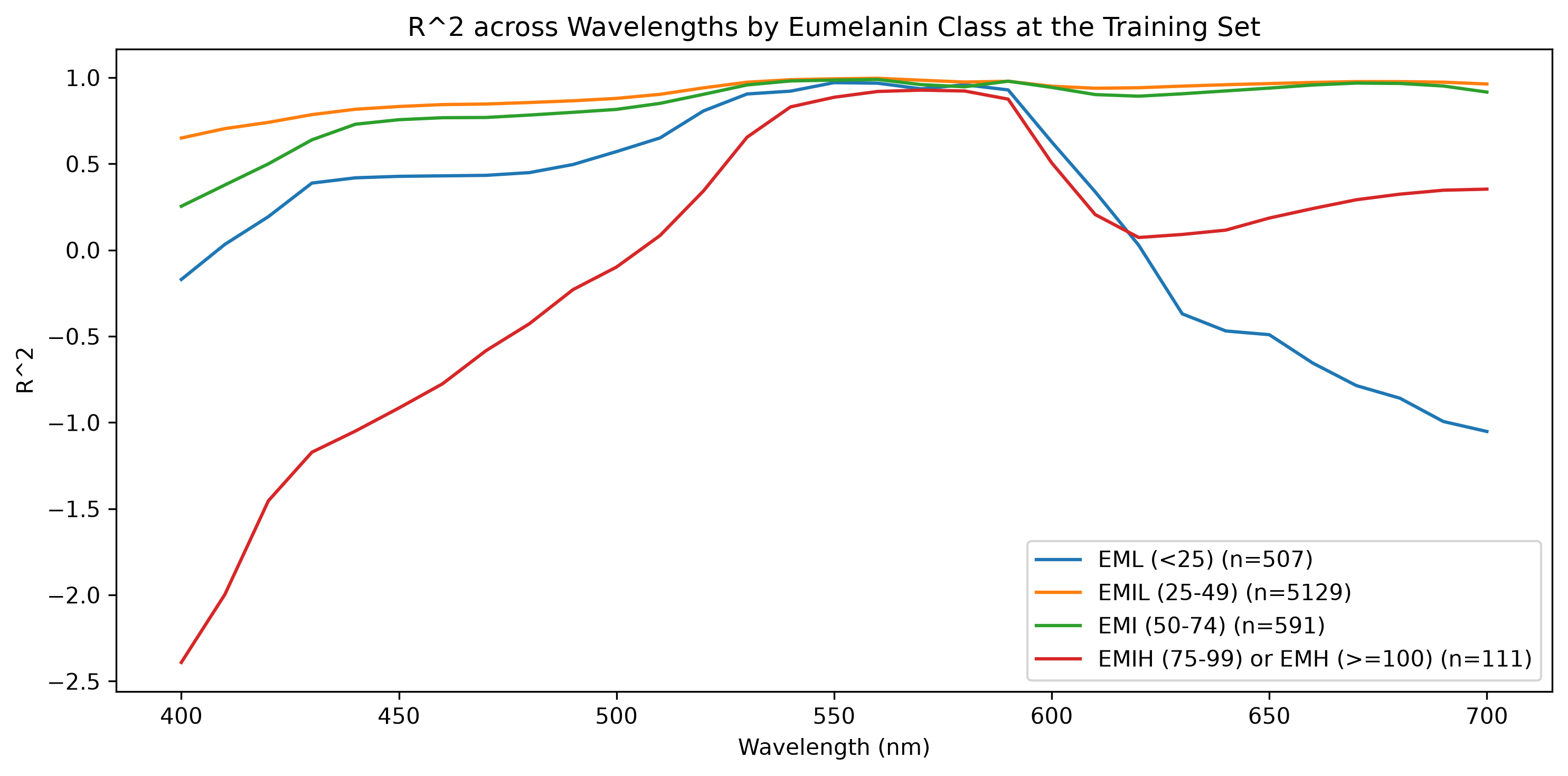
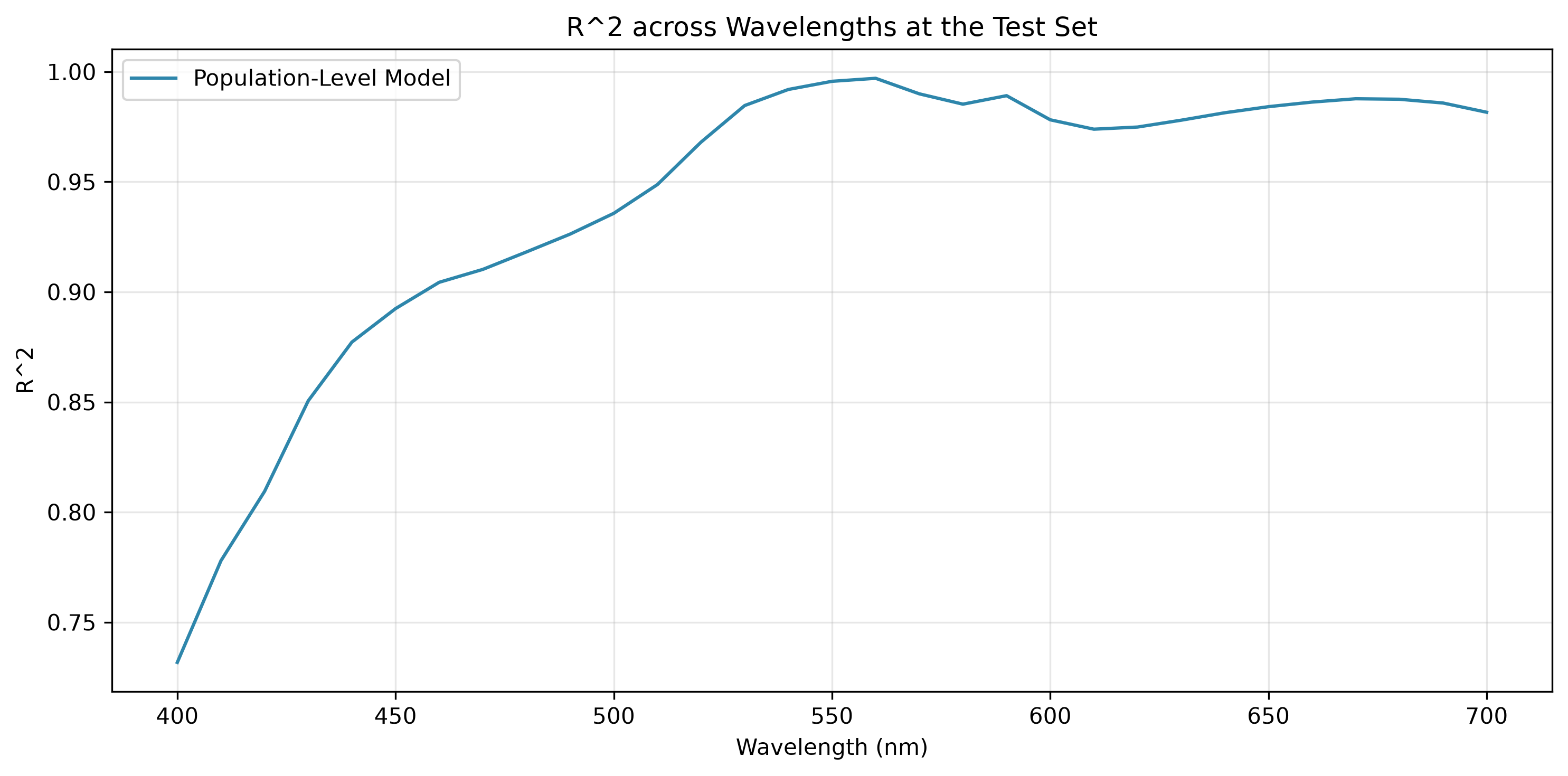
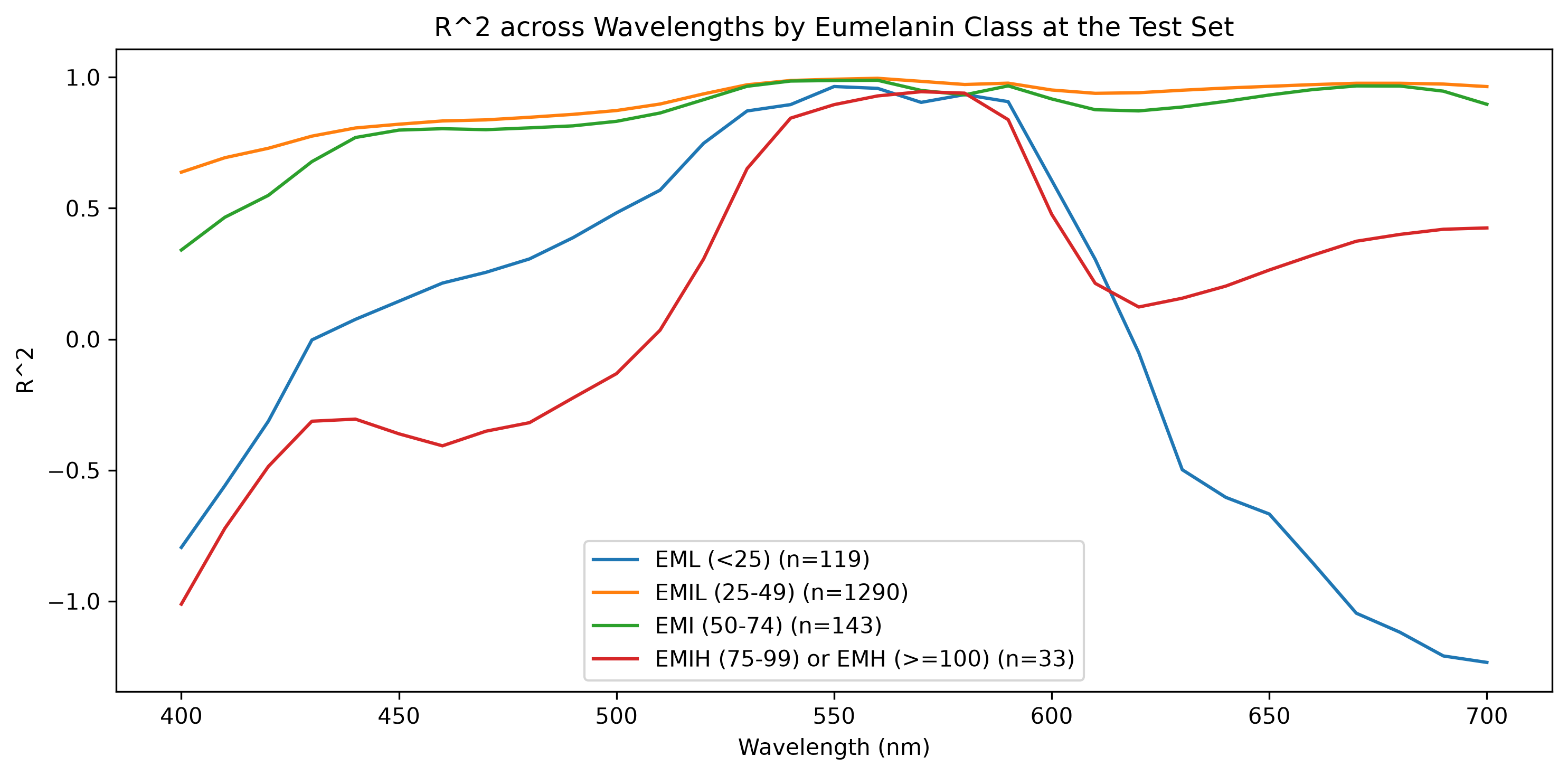
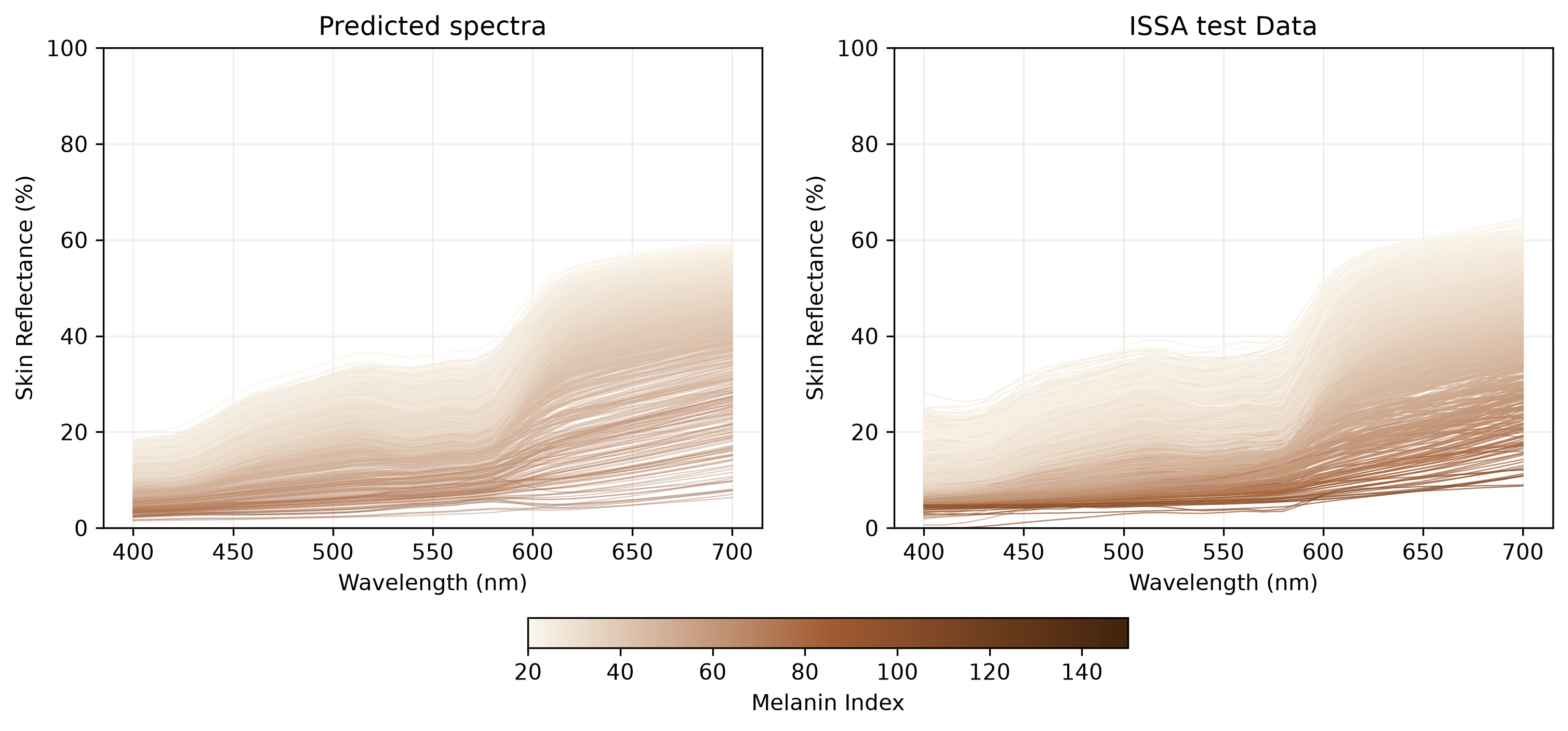
4.2 Evaluation on test data
| Model | R² | RMSE (%) | MAE (%) | |
|---|---|---|---|---|
| 0 | Population-Level (Fixed Effects) | 0.964578 | 1.428091 | 1.06963 |
5 Synthetic spectra generation
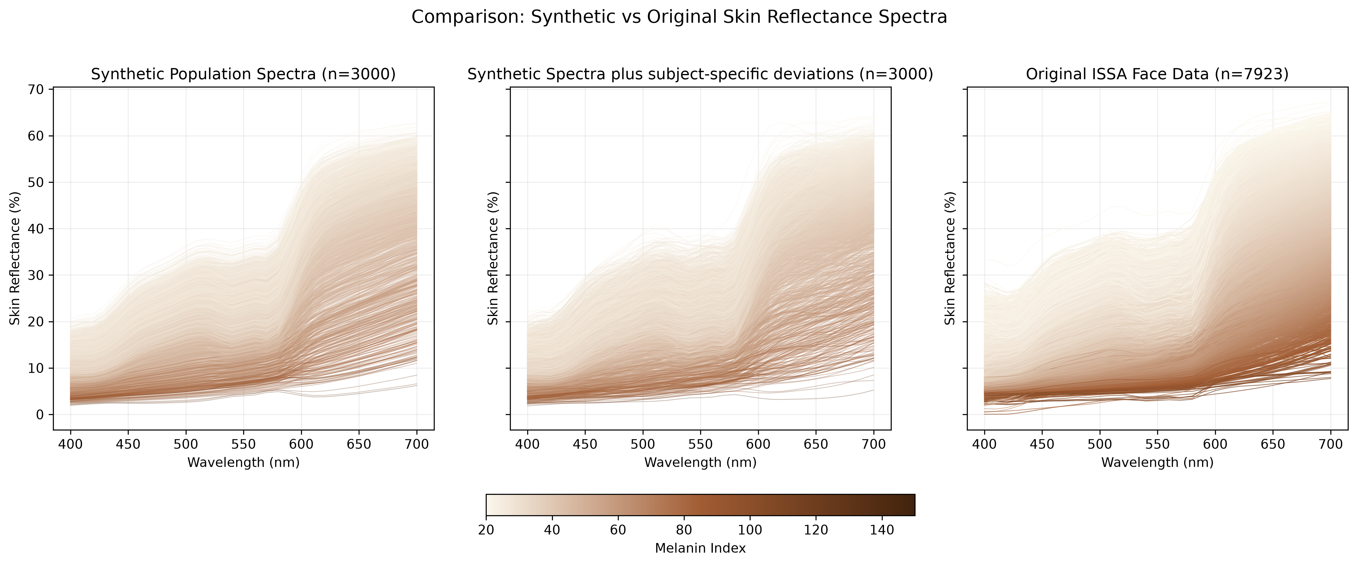
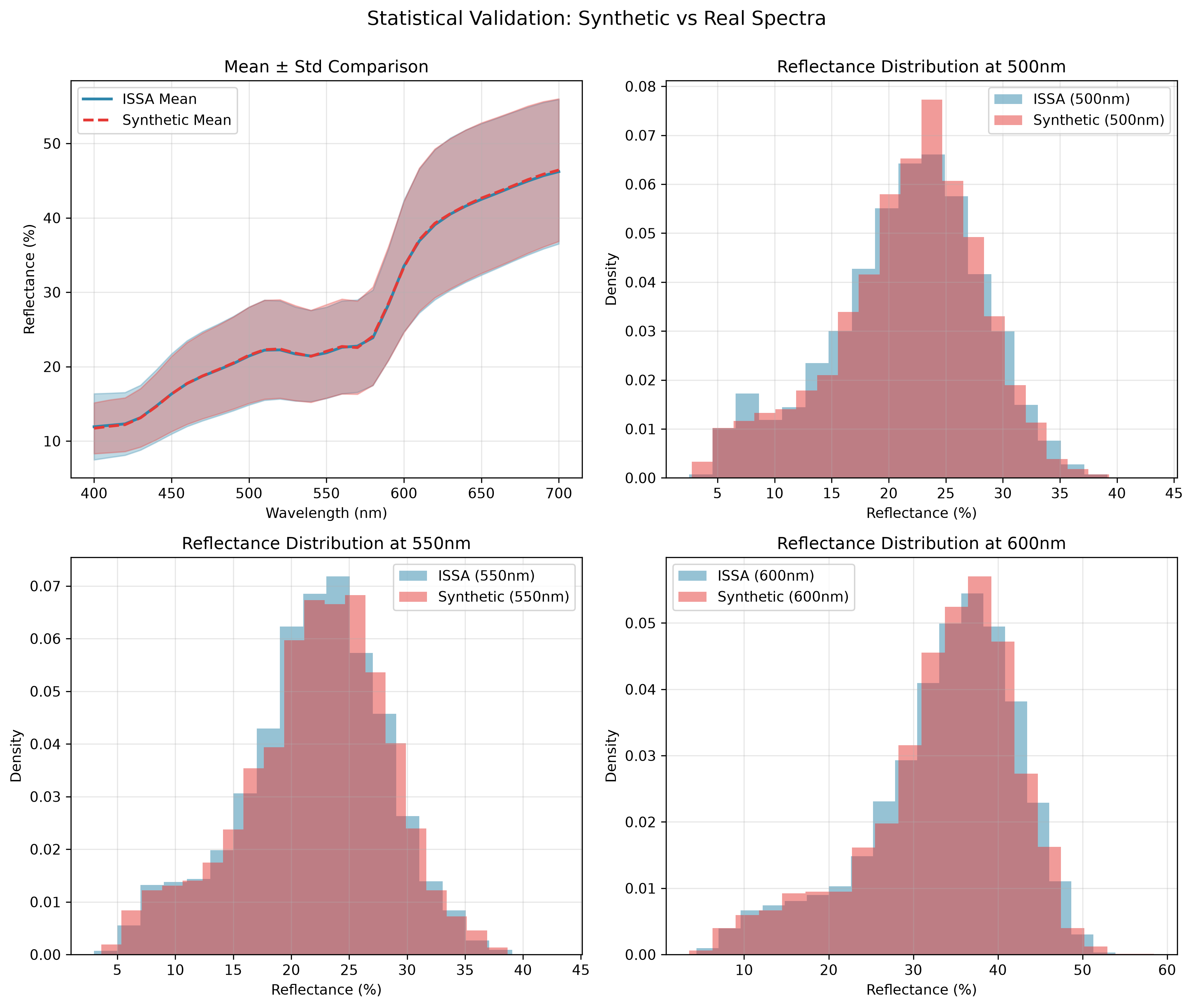
This section demonstrates how to generate realistic synthetic skin reflectance.
Choromophore Index Sampling: Sample melanin variable (MEL) and hemoglobin variable (HEM) pairs from the fitted GMM to ensure biologically plausible combinations.
Spectral Prediction: For each sampled (MEL, HEM) pair, use the BVCM fixed effects (population-level coefficients) to predict the corresponding skin reflectance spectrum. Then add subject-specific random effects to introduce realistic individual variation.
- The new subject-specific deviation \(Z^*\) is sampled from \(p(Z^*\mid Y)=\int p(Z^*\mid Z) p(Z\mid Y) dZ=p(Z^*)\), where the last equality holds as \(Z^*\) is independent to \(Z\).
6 Skin reflectance spectrum filter
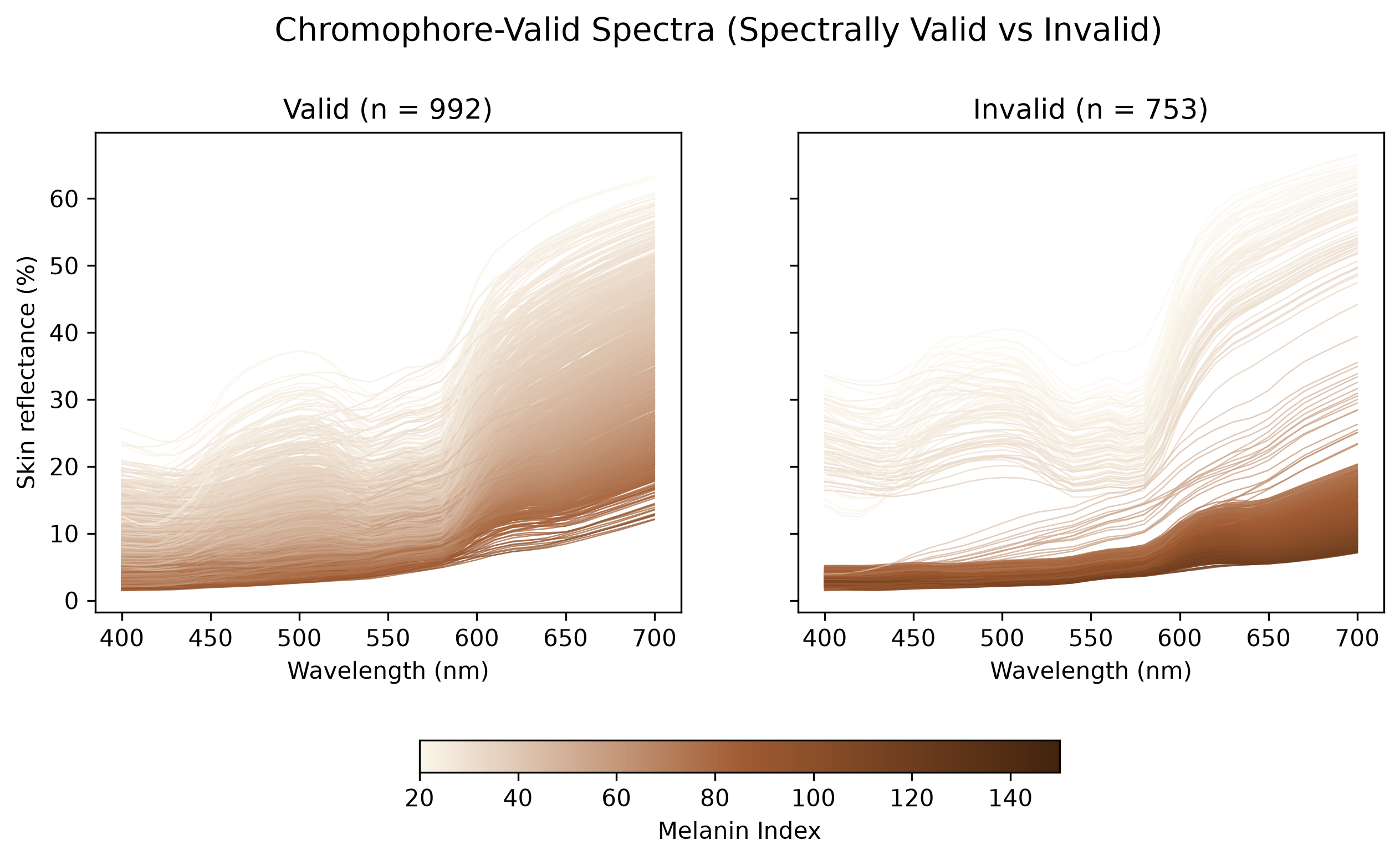
We assess consistency with the ISSA reference data using the existing two-stage procedure:
- Chromophore index validation: compute MI and EI and retain candidates inside at least one component region of the fitted GMM. Each region is bounded by the 99th percentile of the Mahalanobis distances of the ISSA facial spectra assigned to that component.
- Spectral assessment: among Stage 1 candidates, retain spectra whose BVCM residual Mahalanobis distance does not exceed the 95th percentile of the distances of all cleaned ISSA facial spectra, computed under the BVCM refitted to those same spectra.
Rejection indicates inconsistency with this ISSA reference under these criteria. It does not establish biological implausibility or distinguish missing empirical coverage from other causes.
6.1 Validation reference: BVCM refitted to all ISSA facial spectra
The training-split fit above is used only for model evaluation. For validation, the BVCM is refitted to all cleaned facial spectra with the same priors and sampler settings, and the Stage 2 threshold is the in-sample 95th percentile of their Mahalanobis distances. In-sample calibration is justified by the stability of the fit: the population-level RMSE on the held-out test spectra is essentially equal to that on the training spectra.
Loaded compatible full-data Gibbs checkpoint: bvcm_gibbs_full_reference_checkpoint.npz
Full-data posterior means: length scale=45.383482, amplitude=0.108663, noise variance=0.00023009
Acceptance rate: 13.55%
Population-level RMSE on all 7923 spectra: full-data fit 1.417, training-split fit 1.415
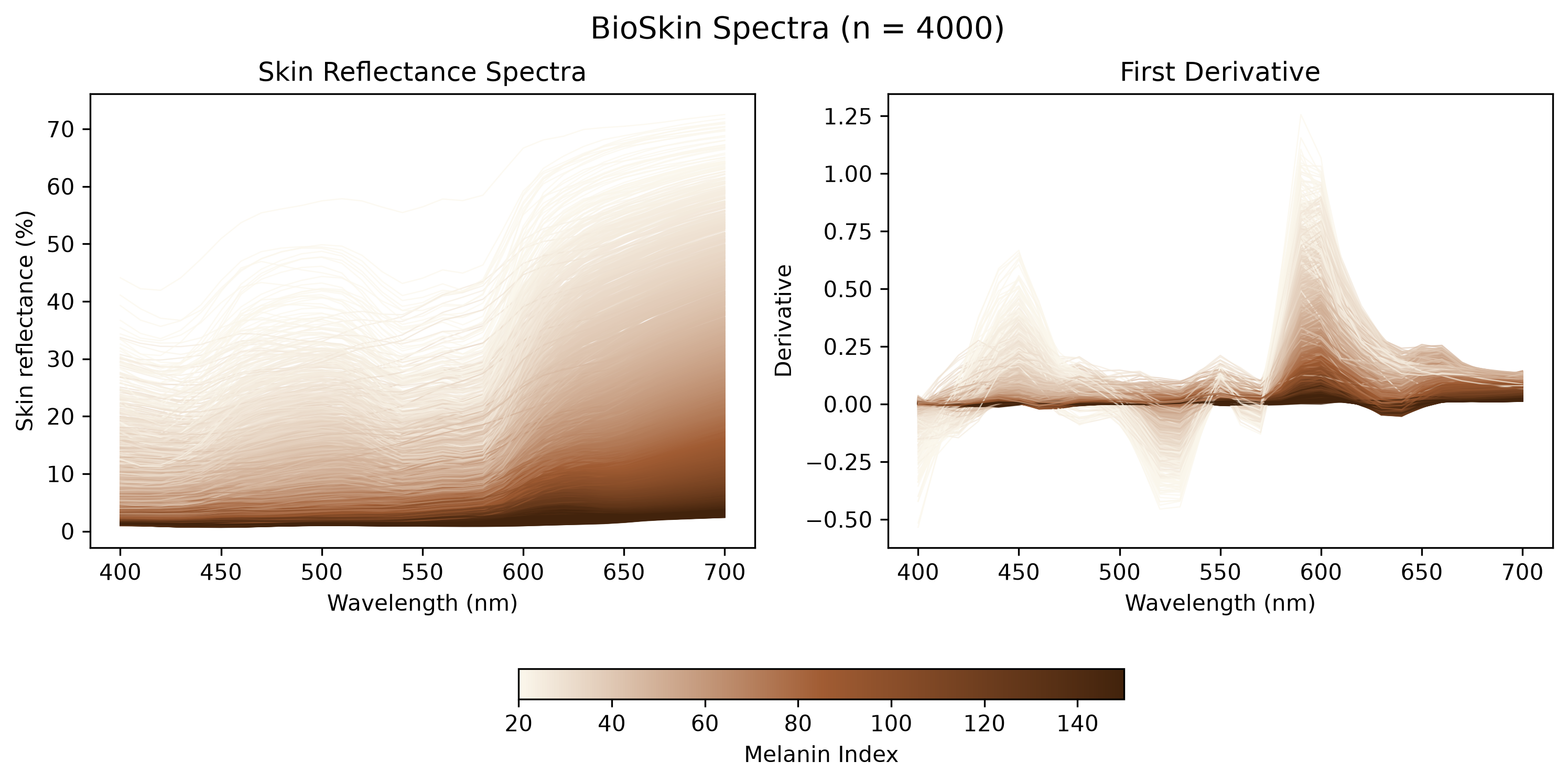
6.1.1 Corrected BioSkin inputs
This section uses Carlos’s corrected 4,000-spectrum dataset in bioskin_data/. The network-ready CSV places melanin type ratio in column 4 and blood oxygenation in column 5 (one-based). The physical-units CSV has its own named column order. Parameter plots use the physical values, with thickness expressed in micrometres.
The input loader checks row counts, parameter scaling and slot order, finite reflectance fractions, and exact wavelength alignment. Reflectance is converted to percentages once. The existing GMM and BVCM validation criteria are unchanged. Execute the notebook with the ISSA workbook available to obtain updated validation results.
Loaded 4,000 corrected BioSkin spectra at 31 ISSA wavelengths.
Reflectance range: 0.6830% to 72.5010%| count | mean | std | min | 25% | 50% | 75% | max | |
|---|---|---|---|---|---|---|---|---|
| Melanin volume fraction | 4000.0 | 0.214655 | 0.124476 | 0.001223 | 0.106036 | 0.213578 | 0.324239 | 0.429899 |
| Blood volume fraction | 4000.0 | 0.099230 | 0.057012 | 0.001063 | 0.049932 | 0.099178 | 0.147731 | 0.199995 |
| Thickness (micrometres) | 4000.0 | 150.322165 | 57.526798 | 50.002600 | 99.782725 | 151.557250 | 199.059950 | 249.893200 |
| Melanin type ratio | 4000.0 | 0.725285 | 0.043141 | 0.650019 | 0.687451 | 0.726239 | 0.762529 | 0.799992 |
| Blood oxygenation | 4000.0 | 0.950499 | 0.029105 | 0.900002 | 0.925313 | 0.950867 | 0.975665 | 0.999956 |

6.2 PCA comparison of ISSA, BVCM predictions, and BioSkin spectra
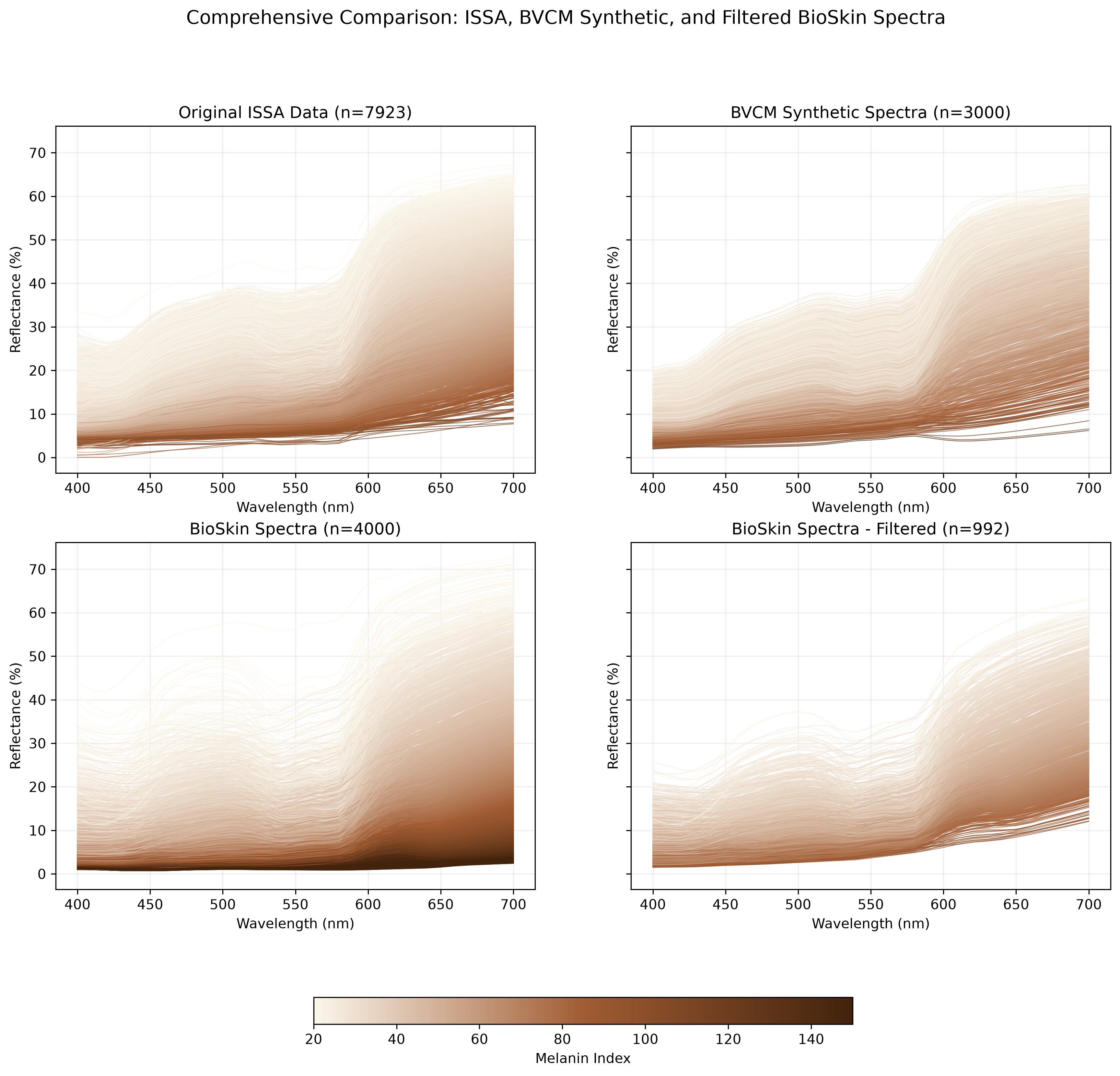
To compare spectral variation on a common basis, we fit PCA to the real ISSA face spectra and project the BVCM population-level predictions and the BioSkin bioskin_spectra onto the resulting components. This reference-based approach keeps the axes directly comparable: overlap with the ISSA score distribution indicates that a dataset reproduces the dominant empirical modes of variation, whereas displacement or dispersion outside the ISSA 95% score ellipse identifies systematic differences. BioSkin reflectance is already converted to percentages when loaded, so all three inputs use the same scale.
| Dataset | n | PC1 mean | PC1 SD | PC2 mean | PC2 SD | Centroid distance from ISSA | Within ISSA 95% region (%) | |
|---|---|---|---|---|---|---|---|---|
| 0 | Real ISSA face data | 7923 | 0.00 | 41.01 | 0.00 | 8.42 | 0.00 | 93.4 |
| 1 | BVCM predicted reflectance | 3000 | 0.53 | 39.31 | 0.43 | 7.80 | 0.05 | 95.4 |
| 2 | BioSkin spectra | 4000 | -107.53 | 51.16 | -5.51 | 10.86 | 2.70 | 22.8 |
The first two ISSA components explain 98.55% of spectral variance.
Corrected BioSkin spectra within the ISSA PC1-PC2 95% score ellipse: 22.78%.
This PCA comparison is descriptive and is separate from the two-stage validation decision.
6.3 Stage 1: Chromophore index validation
6.4 Stage 2: Spectral plausibility assessment
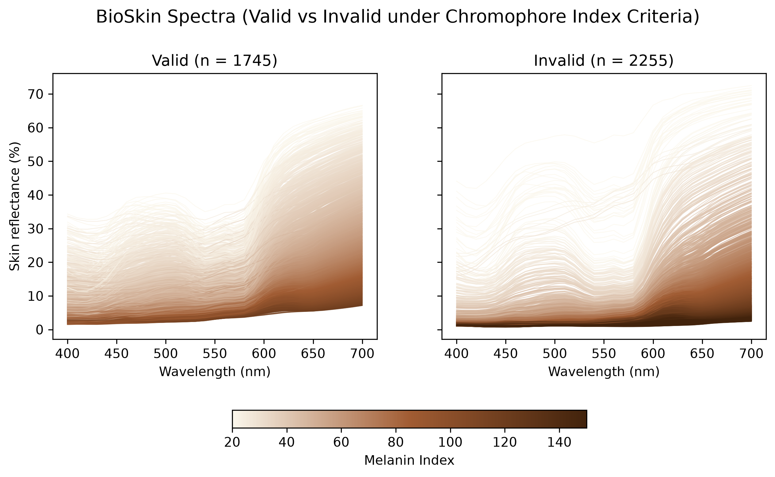
6.5 BioSkin spectra validation overview
6.6 Validation results summary
======================================================================
TWO-STAGE VALIDATION FILTER SUMMARY
======================================================================

Stage 1: Chromophore Index Validation (GMM 99th-percentile regions)
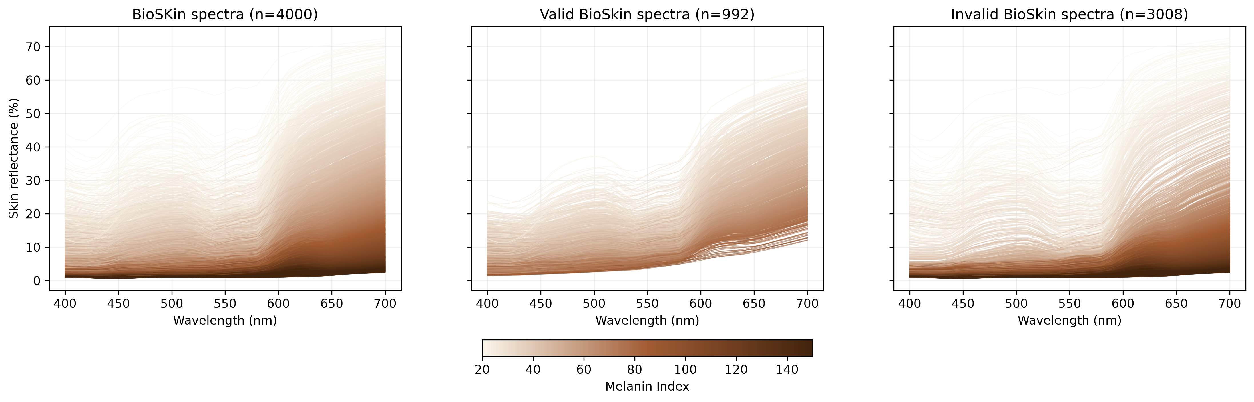
  Input spectra: 4000
  Valid (within GMM): 1745 (43.6%)
  Invalid (outside GMM): 2255 (56.4%)

Stage 2: Spectral Plausibility Assessment (Mahalanobis Distance)
  Input (from Stage 1): 1745
  Threshold: 9.35 (in-sample 95th percentile, all ISSA facial spectra)
  Valid (plausible spectra): 992 (56.8%)
  Invalid (implausible spectra): 753 (43.2%)

Overall Filter Performance:
  Total input: 4000
  Total valid: 992 (24.8%)
  Total rejected: 3008 (75.2%)

Chromophore Index Statistics (Valid Spectra):
  Melanin Index: [20.85, 97.97]
  Erythema Index: [16.79, 56.36]
======================================================================
Validation results saved to D:\THUCloud\Seafile\SkinSpectra\SkinSim_Quarto\output\corrected_validation