summer-winter
Tina Lasisi
2025-03-09 16:42:01
Last updated: 2025-03-09
Checks: 6 1
Knit directory: SAPPHIRE/
This reproducible R Markdown analysis was created with workflowr (version 1.7.1). The Checks tab describes the reproducibility checks that were applied when the results were created. The Past versions tab lists the development history.
The R Markdown file has unstaged changes. To know which version of
the R Markdown file created these results, you’ll want to first commit
it to the Git repo. If you’re still working on the analysis, you can
ignore this warning. When you’re finished, you can run
wflow_publish to commit the R Markdown file and build the
HTML.
Great job! The global environment was empty. Objects defined in the global environment can affect the analysis in your R Markdown file in unknown ways. For reproduciblity it’s best to always run the code in an empty environment.
The command set.seed(20240923) was run prior to running
the code in the R Markdown file. Setting a seed ensures that any results
that rely on randomness, e.g. subsampling or permutations, are
reproducible.
Great job! Recording the operating system, R version, and package versions is critical for reproducibility.
Nice! There were no cached chunks for this analysis, so you can be confident that you successfully produced the results during this run.
Great job! Using relative paths to the files within your workflowr project makes it easier to run your code on other machines.
Great! You are using Git for version control. Tracking code development and connecting the code version to the results is critical for reproducibility.
The results in this page were generated with repository version 3460f1b. See the Past versions tab to see a history of the changes made to the R Markdown and HTML files.
Note that you need to be careful to ensure that all relevant files for
the analysis have been committed to Git prior to generating the results
(you can use wflow_publish or
wflow_git_commit). workflowr only checks the R Markdown
file, but you know if there are other scripts or data files that it
depends on. Below is the status of the Git repository when the results
were generated:
Ignored files:
    Ignored:    .DS_Store
    Ignored:    .Rhistory
    Ignored:    .Rproj.user/
    Ignored:    data/.DS_Store
    Ignored:    output/.DS_Store

Unstaged changes:
    Modified:   analysis/pigmentationdata.Rmd
    Modified:   analysis/summer-winter.Rmd
    Modified:   output/coeff_plots_summer-winter/coeff_Forehead_B.png
    Modified:   output/coeff_plots_summer-winter/coeff_Forehead_CIE_L.png
    Modified:   output/coeff_plots_summer-winter/coeff_Forehead_CIE_a.png
    Modified:   output/coeff_plots_summer-winter/coeff_Forehead_CIE_b.png
    Modified:   output/coeff_plots_summer-winter/coeff_Forehead_E.png
    Modified:   output/coeff_plots_summer-winter/coeff_Forehead_G.png
    Modified:   output/coeff_plots_summer-winter/coeff_Forehead_M.png
    Modified:   output/coeff_plots_summer-winter/coeff_Forehead_R.png
    Modified:   output/coeff_plots_summer-winter/coeff_LeftUpperInnerArm_B.png
    Modified:   output/coeff_plots_summer-winter/coeff_LeftUpperInnerArm_CIE_L.png
    Modified:   output/coeff_plots_summer-winter/coeff_LeftUpperInnerArm_CIE_a.png
    Modified:   output/coeff_plots_summer-winter/coeff_LeftUpperInnerArm_CIE_b.png
    Modified:   output/coeff_plots_summer-winter/coeff_LeftUpperInnerArm_E.png
    Modified:   output/coeff_plots_summer-winter/coeff_LeftUpperInnerArm_G.png
    Modified:   output/coeff_plots_summer-winter/coeff_LeftUpperInnerArm_M.png
    Modified:   output/coeff_plots_summer-winter/coeff_LeftUpperInnerArm_R.png
    Modified:   output/coeff_plots_summer-winter/coeff_RightUpperInnerArm_B.png
    Modified:   output/coeff_plots_summer-winter/coeff_RightUpperInnerArm_CIE_L.png
    Modified:   output/coeff_plots_summer-winter/coeff_RightUpperInnerArm_CIE_a.png
    Modified:   output/coeff_plots_summer-winter/coeff_RightUpperInnerArm_CIE_b.png
    Modified:   output/coeff_plots_summer-winter/coeff_RightUpperInnerArm_E.png
    Modified:   output/coeff_plots_summer-winter/coeff_RightUpperInnerArm_G.png
    Modified:   output/coeff_plots_summer-winter/coeff_RightUpperInnerArm_M.png
    Modified:   output/coeff_plots_summer-winter/coeff_RightUpperInnerArm_R.png
    Modified:   output/withinstats_filtered/Forehead_B.png
    Modified:   output/withinstats_filtered/Forehead_CIE_L.png
    Modified:   output/withinstats_filtered/Forehead_CIE_a.png
    Modified:   output/withinstats_filtered/Forehead_CIE_b.png
    Modified:   output/withinstats_filtered/Forehead_E.png
    Modified:   output/withinstats_filtered/Forehead_G.png
    Modified:   output/withinstats_filtered/Forehead_M.png
    Modified:   output/withinstats_filtered/Forehead_R.png
    Modified:   output/withinstats_filtered/LeftUpperInnerArm_B.png
    Modified:   output/withinstats_filtered/LeftUpperInnerArm_CIE_L.png
    Modified:   output/withinstats_filtered/LeftUpperInnerArm_CIE_a.png
    Modified:   output/withinstats_filtered/LeftUpperInnerArm_CIE_b.png
    Modified:   output/withinstats_filtered/LeftUpperInnerArm_E.png
    Modified:   output/withinstats_filtered/LeftUpperInnerArm_G.png
    Modified:   output/withinstats_filtered/LeftUpperInnerArm_M.png
    Modified:   output/withinstats_filtered/LeftUpperInnerArm_R.png
    Modified:   output/withinstats_filtered/RightUpperInnerArm_B.png
    Modified:   output/withinstats_filtered/RightUpperInnerArm_CIE_L.png
    Modified:   output/withinstats_filtered/RightUpperInnerArm_CIE_a.png
    Modified:   output/withinstats_filtered/RightUpperInnerArm_CIE_b.png
    Modified:   output/withinstats_filtered/RightUpperInnerArm_E.png
    Modified:   output/withinstats_filtered/RightUpperInnerArm_G.png
    Modified:   output/withinstats_filtered/RightUpperInnerArm_M.png
    Modified:   output/withinstats_filtered/RightUpperInnerArm_R.png
Note that any generated files, e.g. HTML, png, CSS, etc., are not included in this status report because it is ok for generated content to have uncommitted changes.
These are the previous versions of the repository in which changes were
made to the R Markdown (analysis/summer-winter.Rmd) and
HTML (docs/summer-winter.html) files. If you’ve configured
a remote Git repository (see ?wflow_git_remote), click on
the hyperlinks in the table below to view the files as they were in that
past version.
| File | Version | Author | Date | Message |
|---|---|---|---|---|
| Rmd | 3460f1b | Tina Lasisi | 2025-03-09 | Updating index page and dates |
| html | 3460f1b | Tina Lasisi | 2025-03-09 | Updating index page and dates |
| Rmd | 9217a86 | Tina Lasisi | 2025-03-07 | Cleaned data and redid analyses |
Introduction
median data
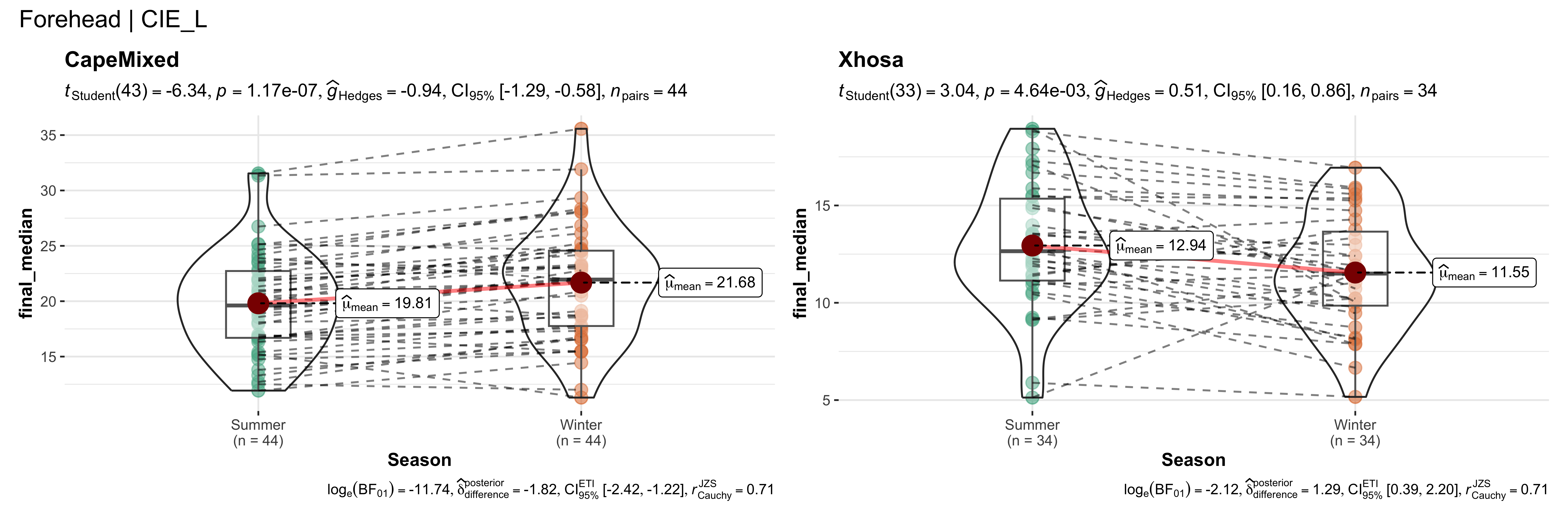
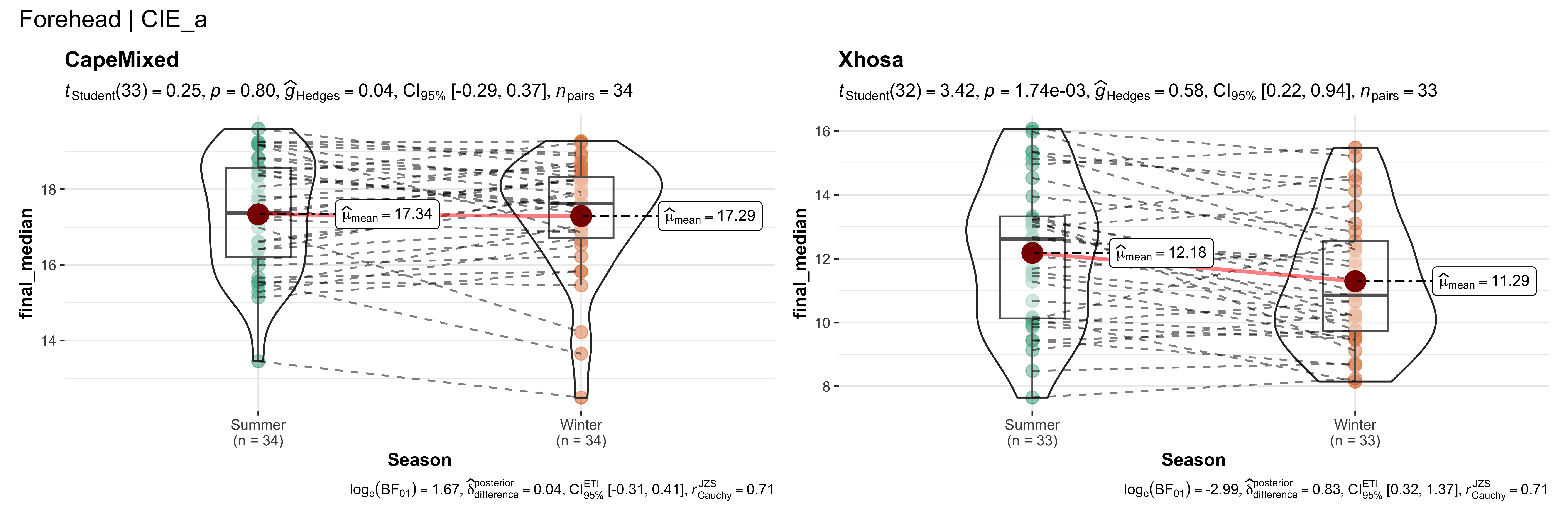
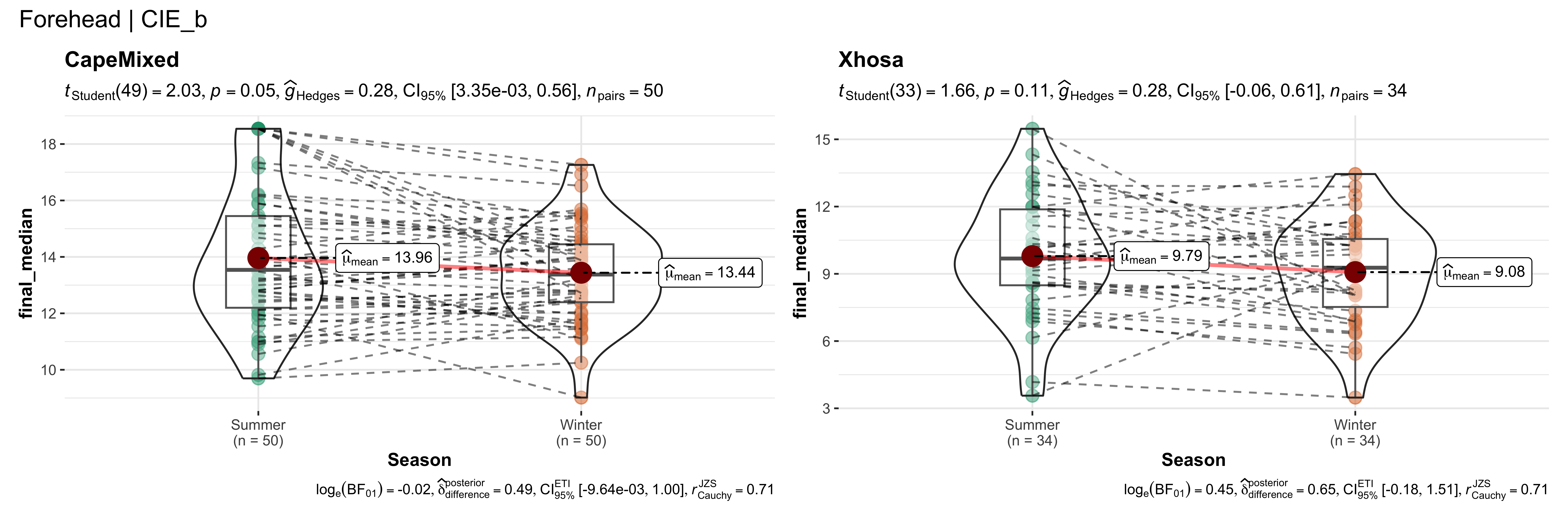
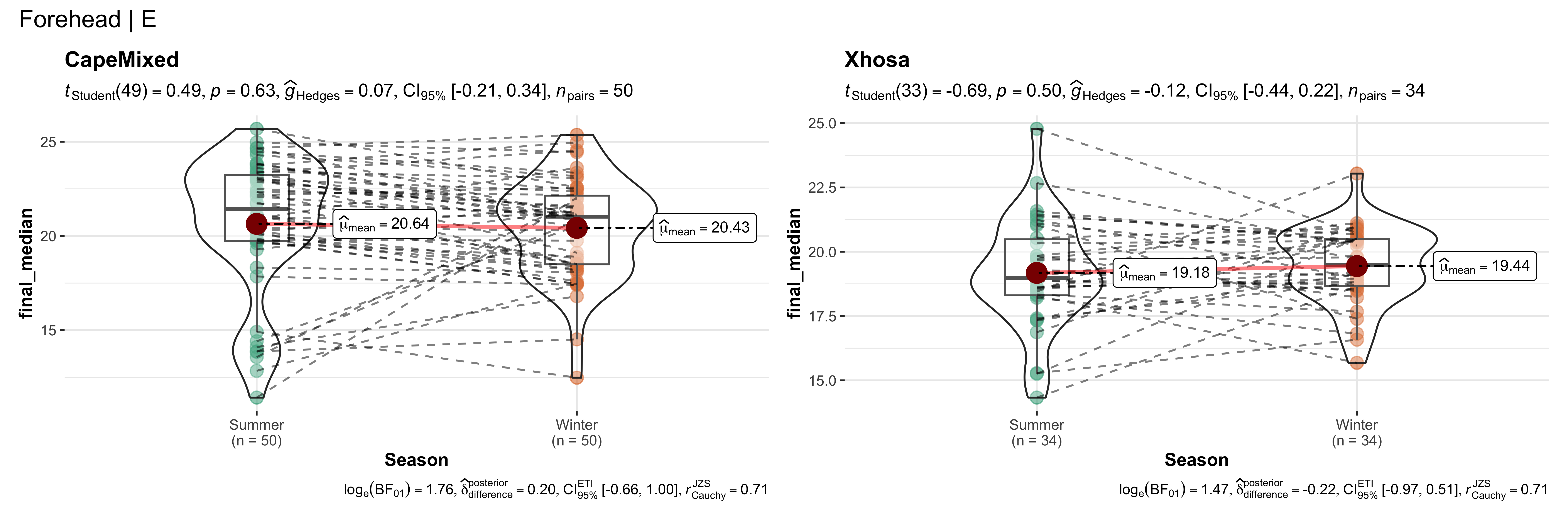
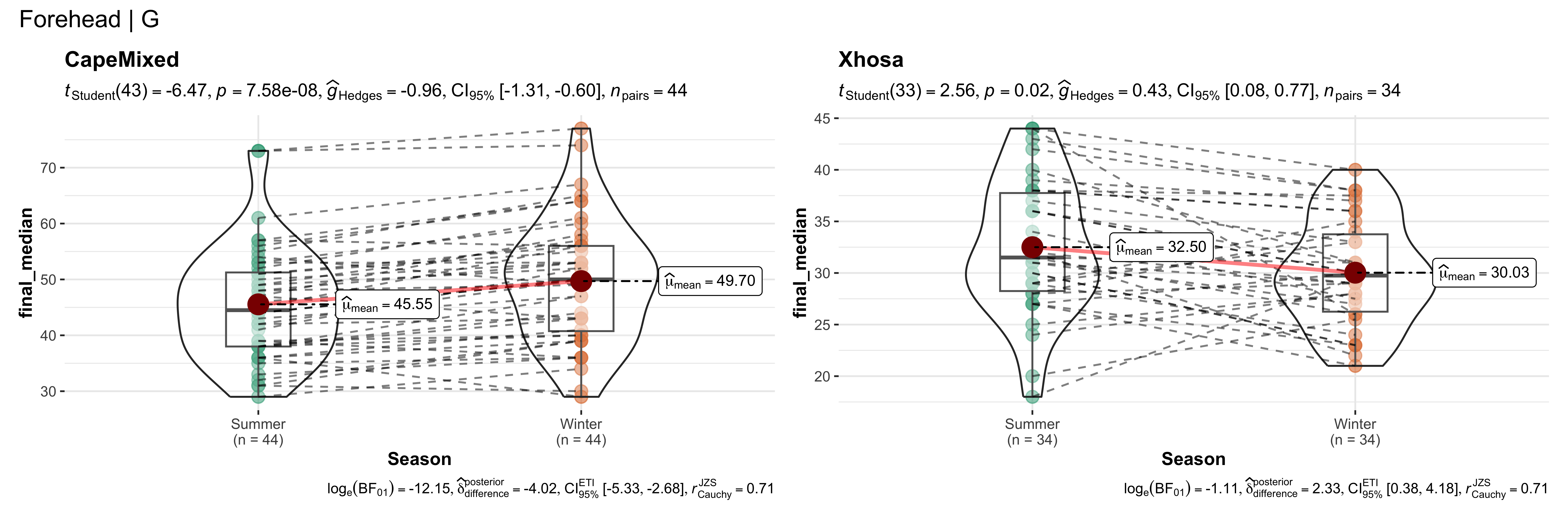
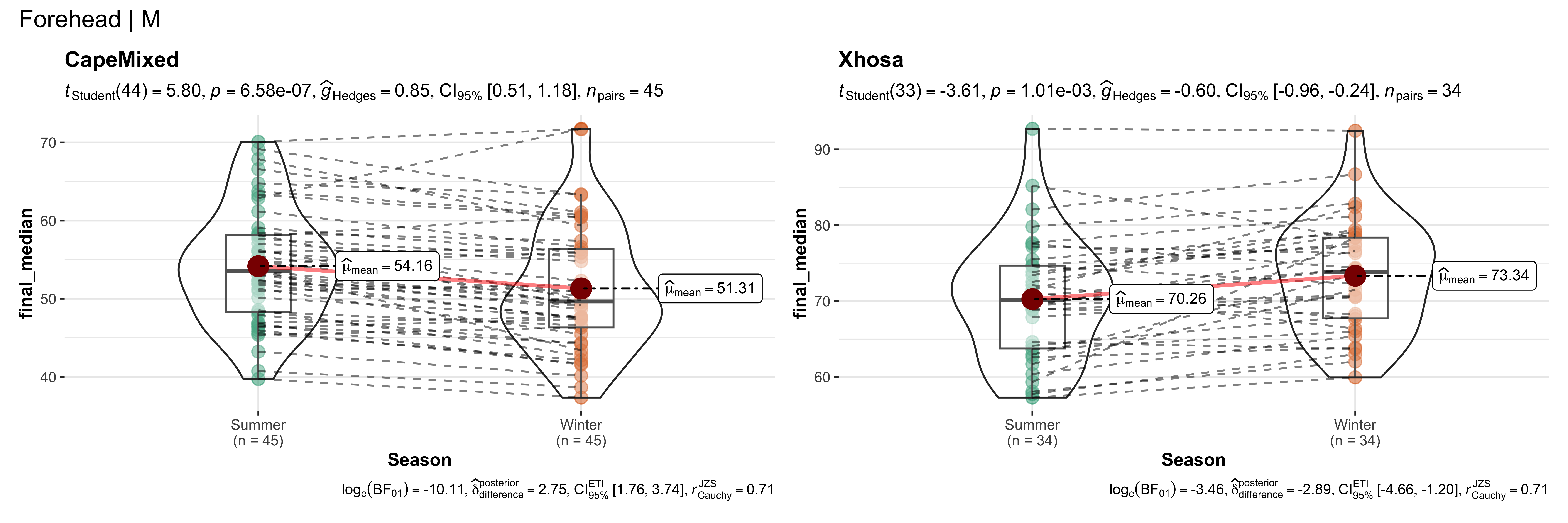
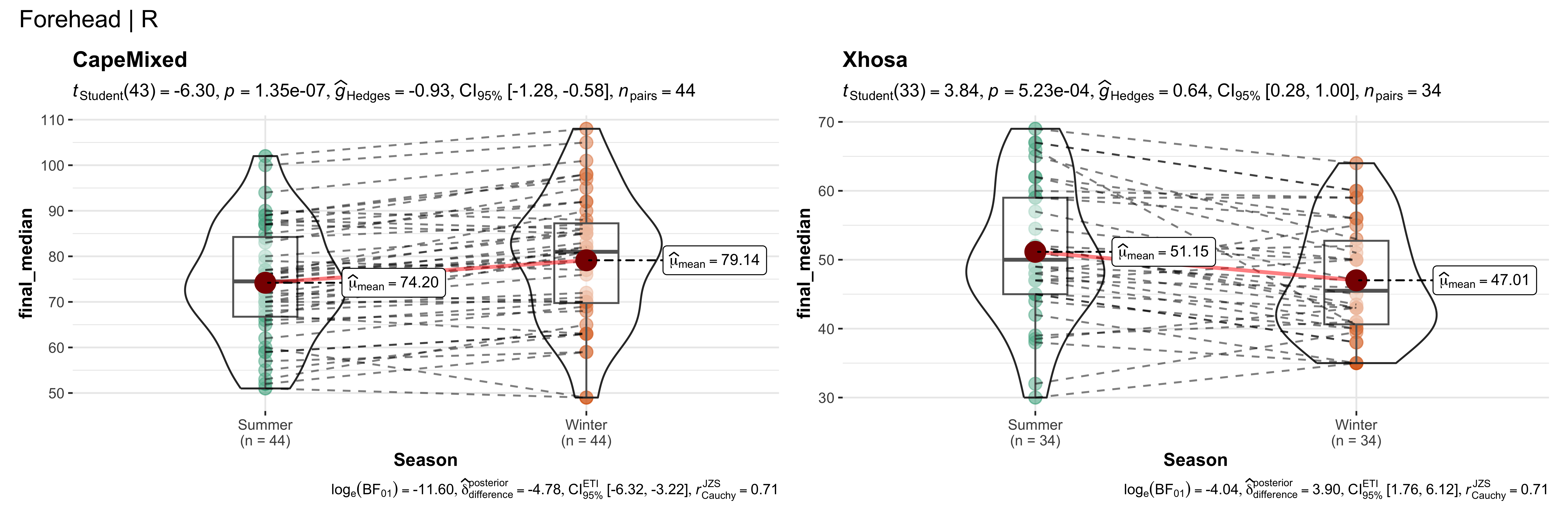
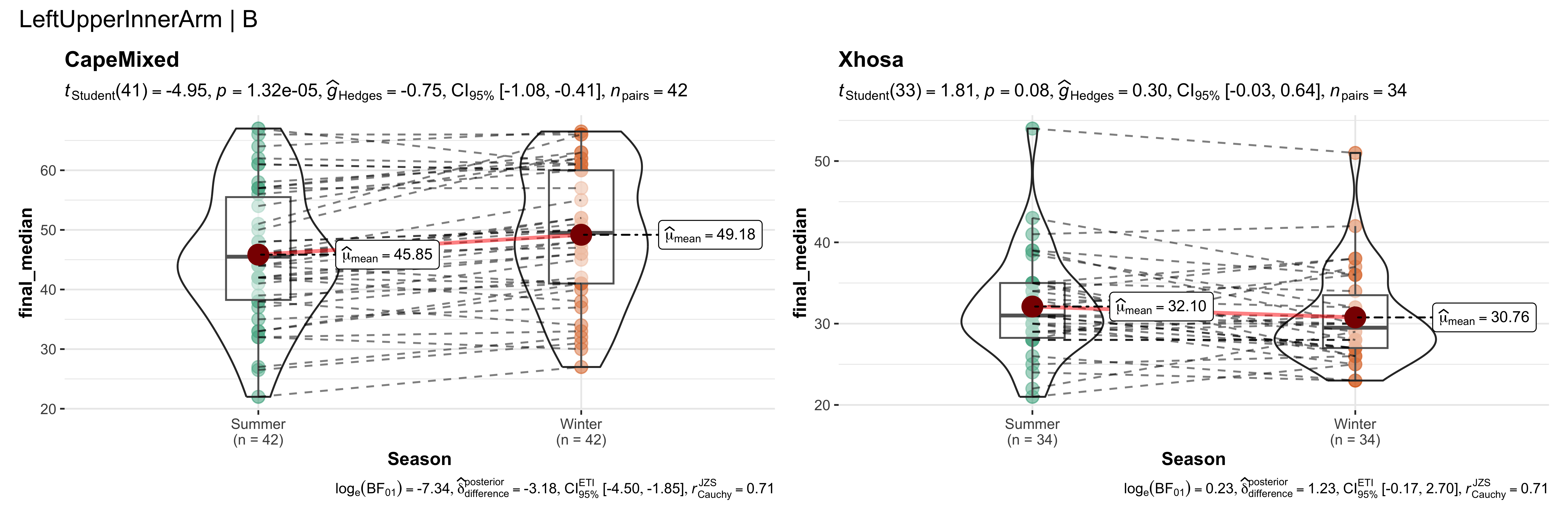
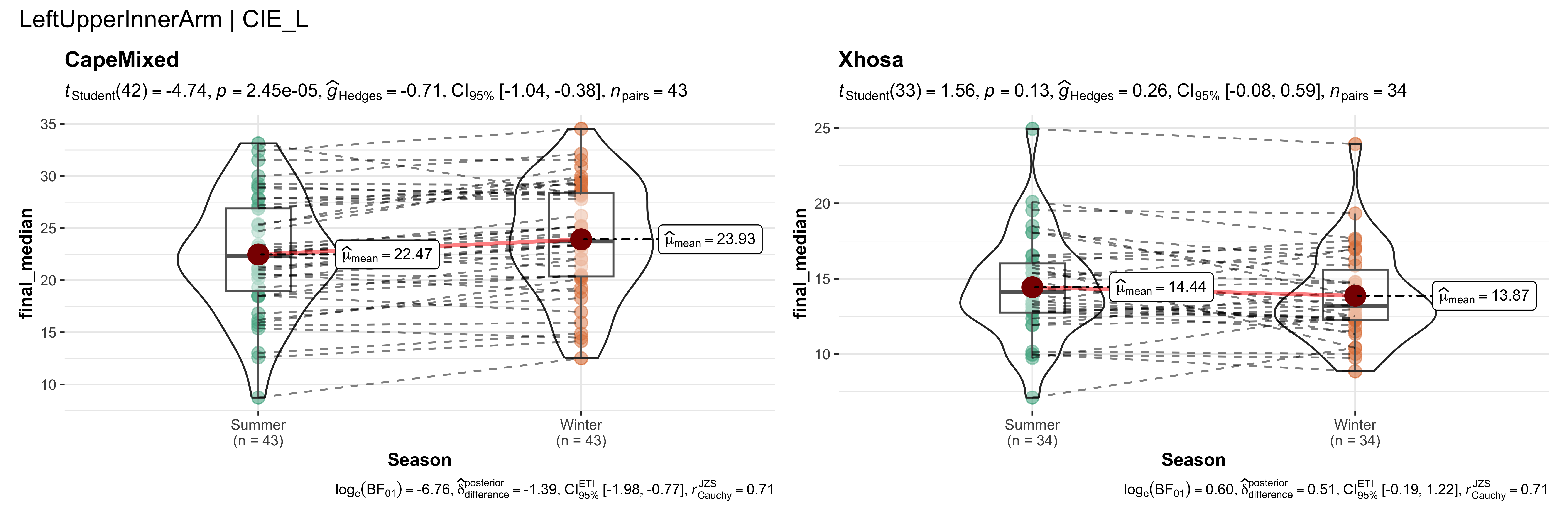
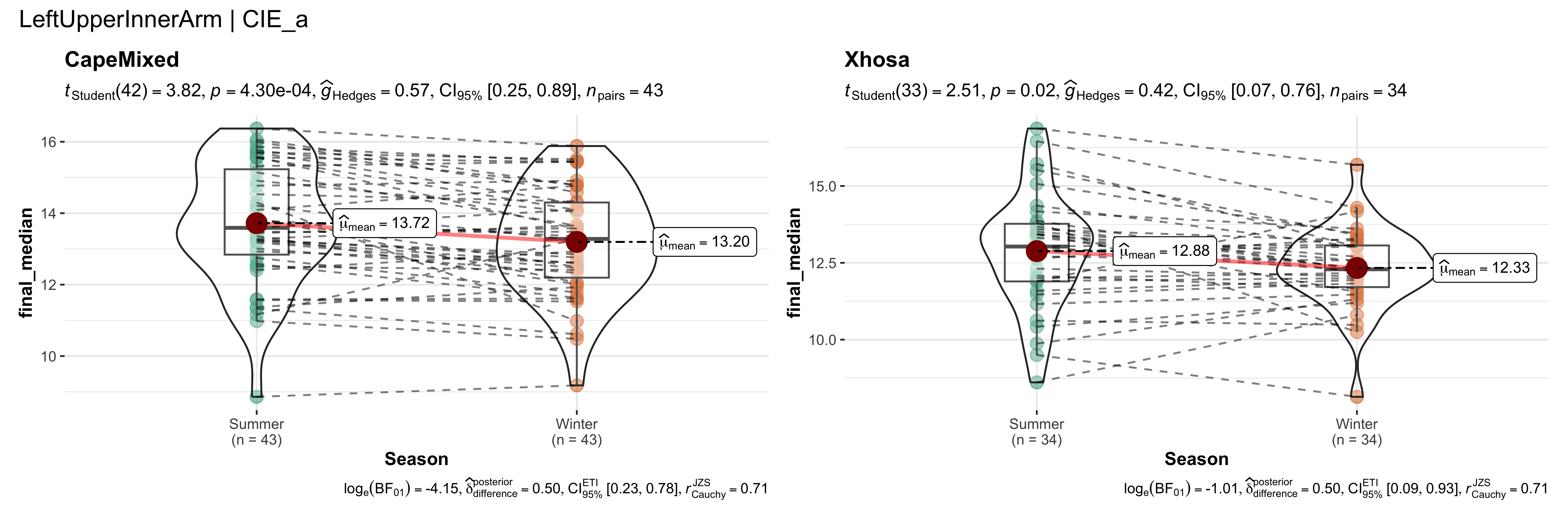
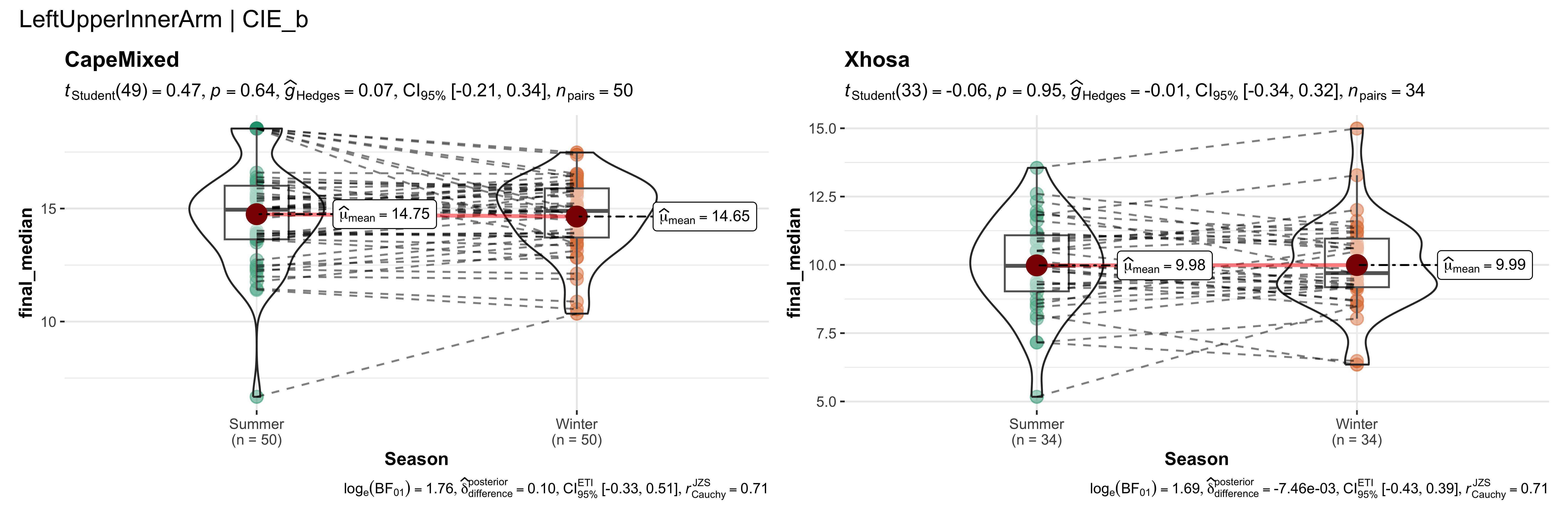
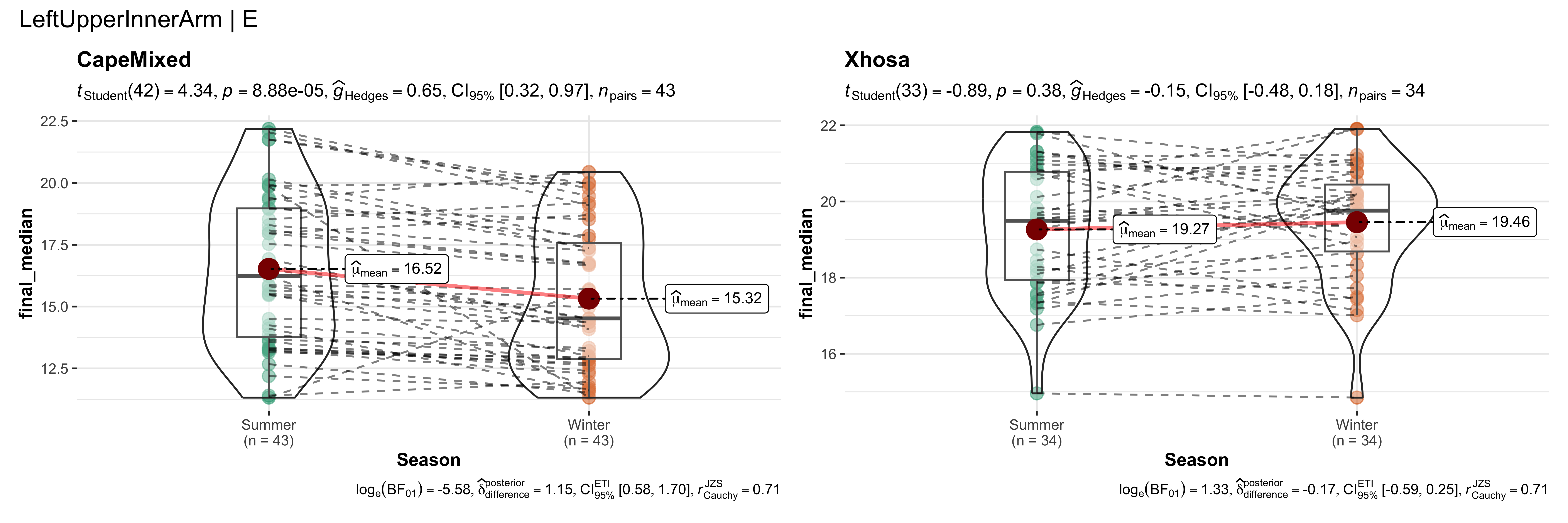
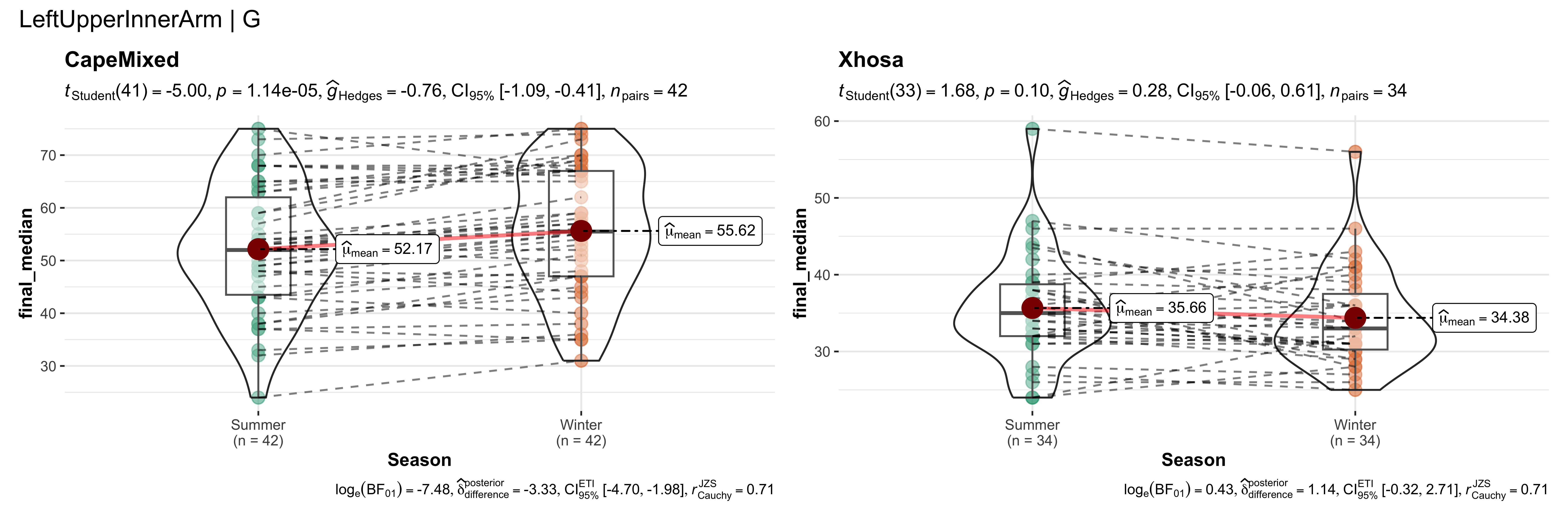
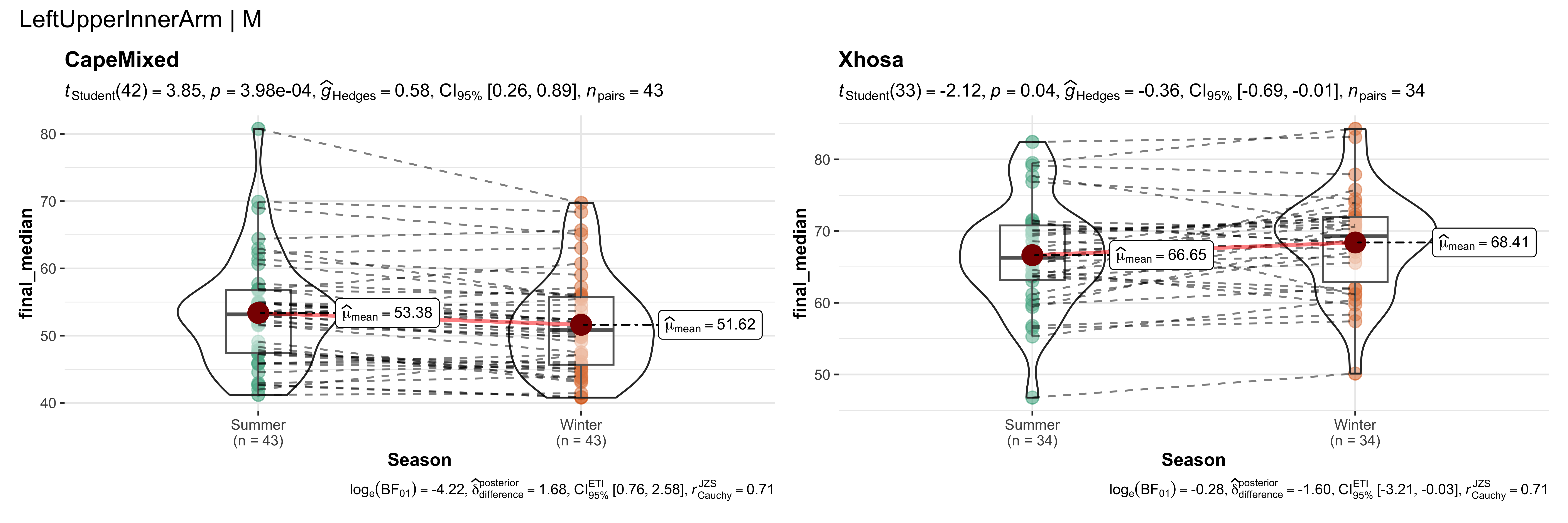
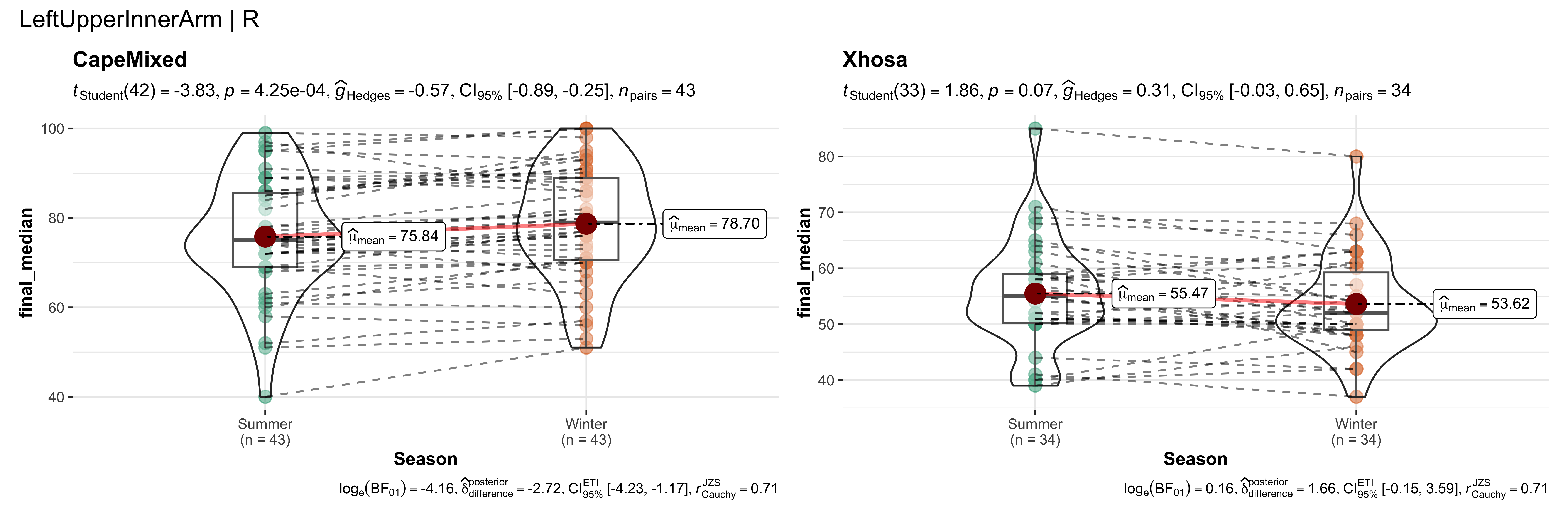
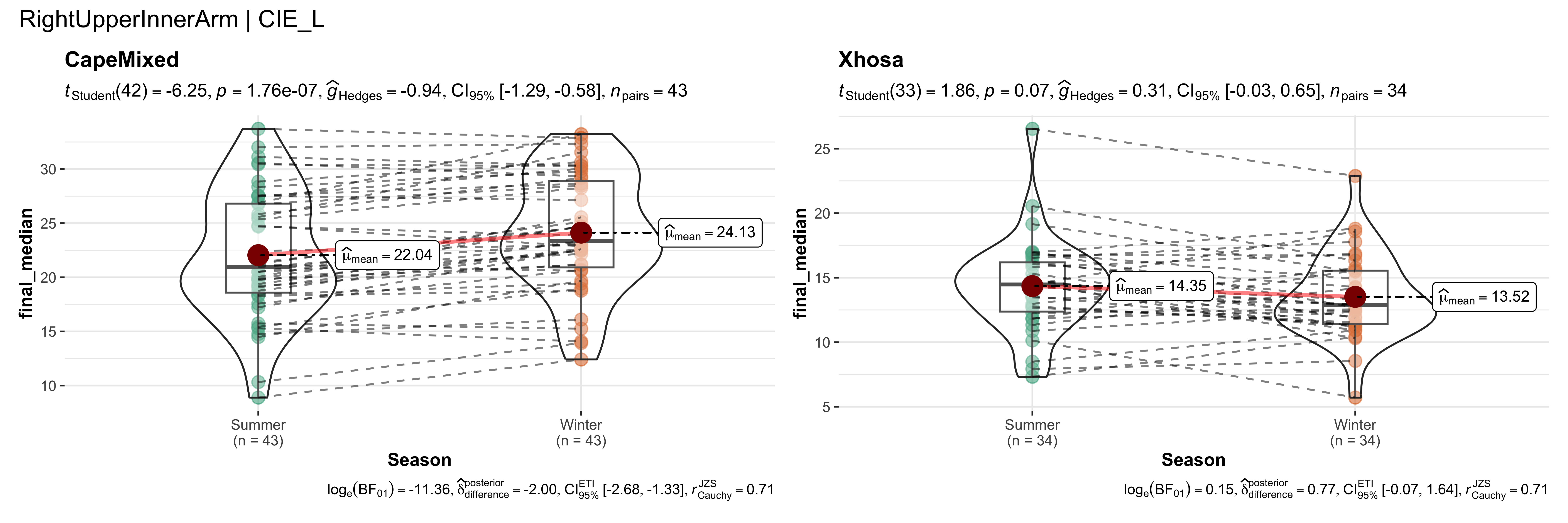
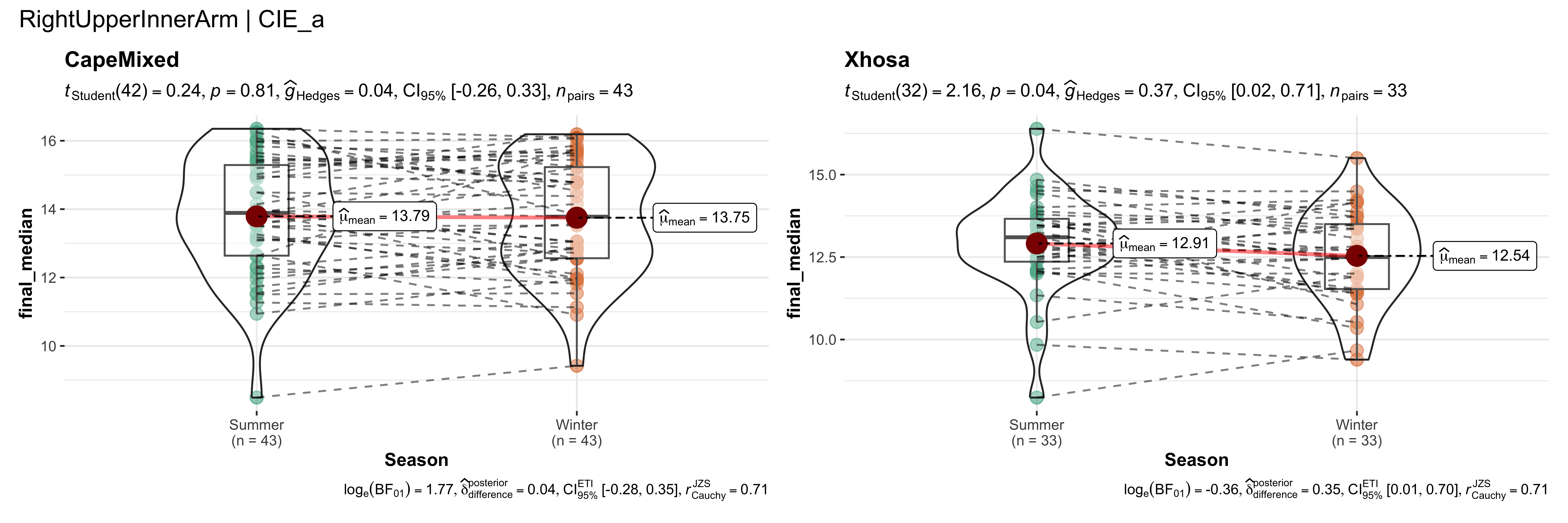
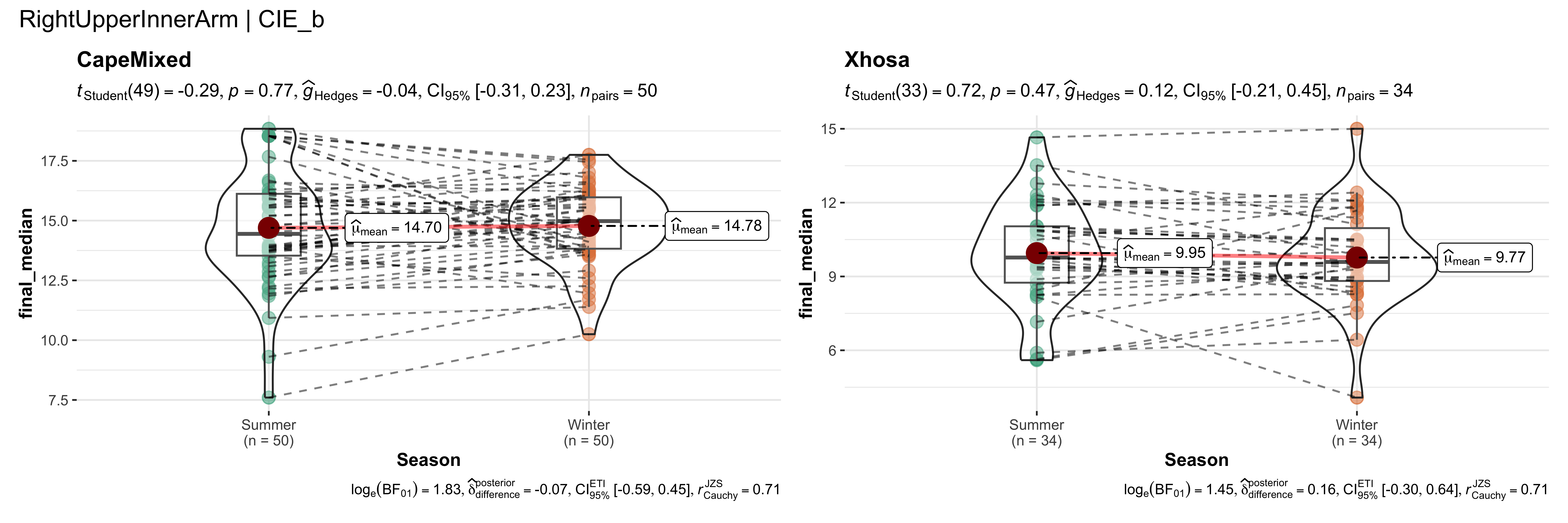
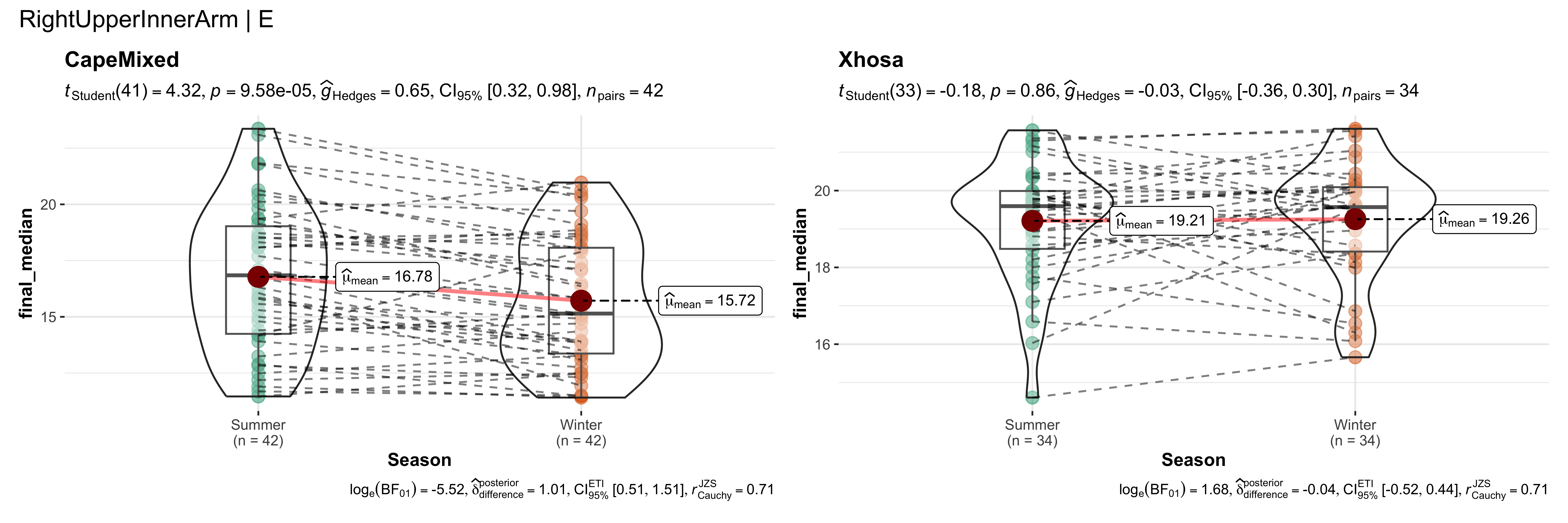
## ---- ensure-both-seasons-and-then-ggwithinstats ----
## This code explicitly filters your data so that each participant has BOTH Summer and Winter
## for each (body_site, measurement_type). We then run grouped_ggwithinstats on that subset.
## This ensures a truly paired analysis with no partial data.
# 1) Read your final medians data, with columns like:
# ParticipantCentreID, Season, Ethnicity, final_median, body_site, measurement_type
df <- read_csv("data/ScreeningDataCollection_medians.csv") |>
filter(Season %in% c("Summer","Winter")) |>
mutate(Season = factor(Season, levels = c("Summer","Winter")))
# 2) Keep only those participants who have BOTH Summer and Winter for each site+metric.
# i.e., for each (ParticipantCentreID, body_site, metric), n_distinct(Season) == 2
df_valid <- df |>
group_by(ParticipantCentreID, body_site, measurement_type) |>
filter(n_distinct(Season) == 2) |>
ungroup()
# 3) Now for each (body_site, measurement_type) combo, we do a grouped_ggwithinstats
# that splits the data by Ethnicity, and does a repeated-measures (paired) test
# comparing Summer vs. Winter.
combos <- df_valid |>
distinct(body_site, measurement_type)
# 4) We'll loop over combos and produce a plot for each
# (If you want a single big combined plot, you'd do a different approach.)
plots <- combos |>
mutate(
plotobj = map2(body_site, measurement_type, ~ {
sub_data <- df_valid |>
filter(body_site == .x, measurement_type == .y)
# If we have no data, skip
if (nrow(sub_data) < 2) return(NULL)
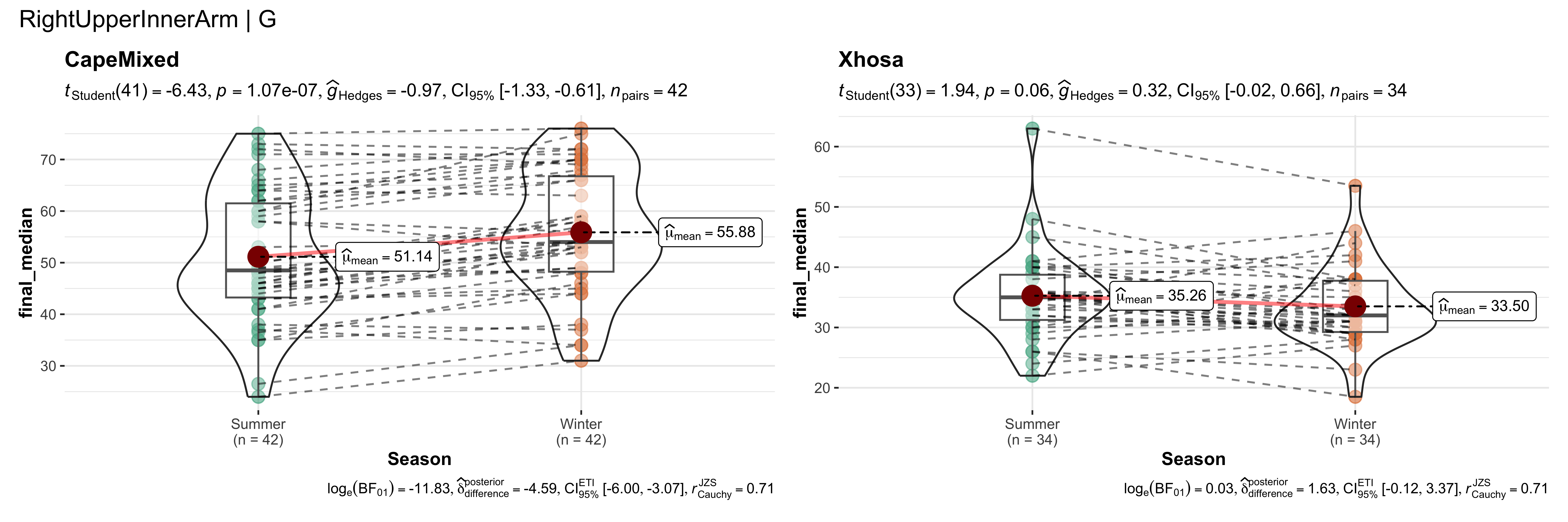
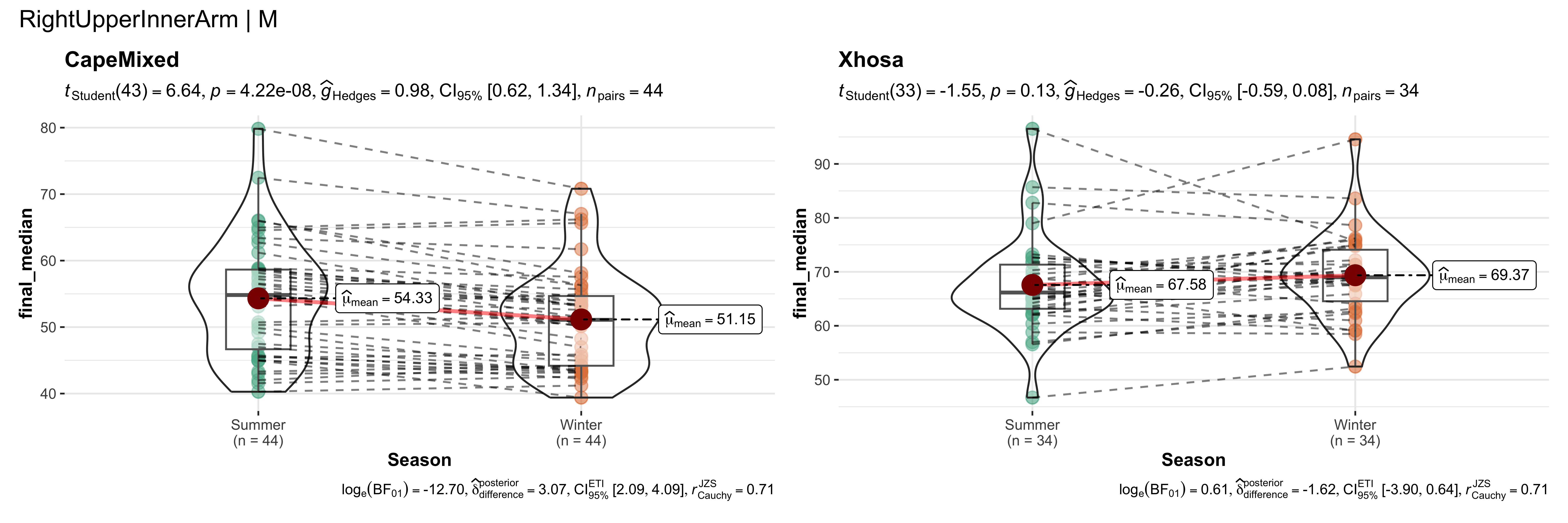
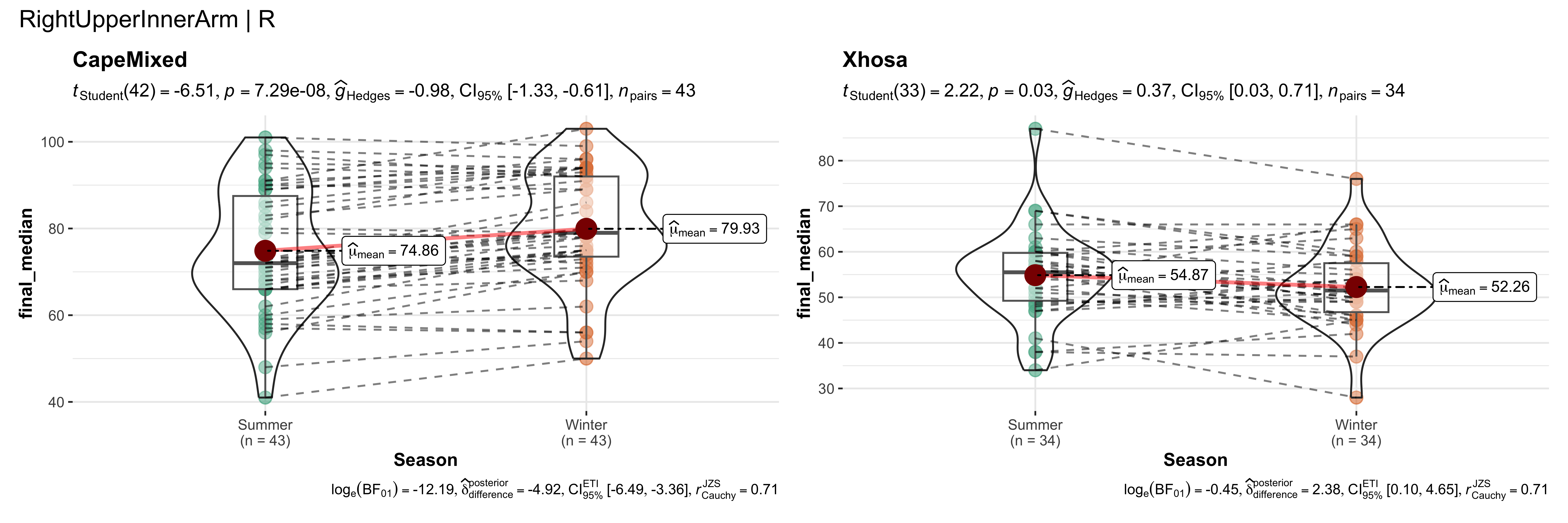
grouped_ggwithinstats(
data = sub_data,
x = Season, # 2-level repeated measure
y = final_median, # numeric outcome
subject.id = ParticipantCentreID,# repeated ID column
grouping.var = Ethnicity, # one subplot per Ethnicity
paired = TRUE, # do a paired test
type = "parametric", # or "nonparametric", etc.
caption.text = "Paired test (Summer vs. Winter) within each Ethnicity",
plotgrid.args= list(ncol = 2), # if you have 2 Ethnicities, side-by-side
annotation.args = list(
title = paste0(.x, " | ", .y)
)
)
})
)
# 5) Save each figure
dir.create("output/withinstats_filtered", showWarnings = FALSE, recursive = TRUE)
plots |>
rowwise() |>
mutate(
outfile = paste0("output/withinstats_filtered/", body_site, "_", measurement_type, ".png"),
saved = {
if (!is.null(plotobj)) {
ggsave(outfile, plotobj, width=12, height=4)
TRUE
} else FALSE
}
) |>
# then print each plot object inline
# or do it in a separate step
ungroup() |>
pull(plotobj) |>
walk(~ if (!is.null(.x)) print(.x))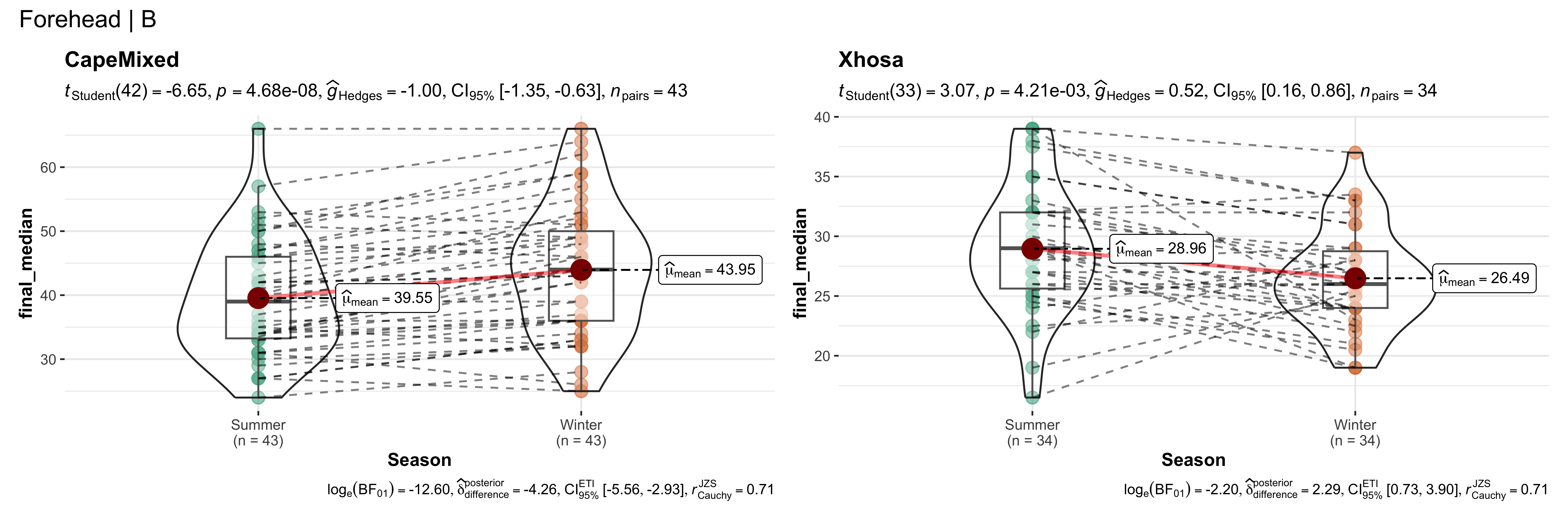

replicate data
stage2_data <- read_csv("data/ScreeningDataCollection_stage2.csv") |>
  group_by(ParticipantCentreID, body_site, measurement_type, Season) |>
  mutate(
    # Subtract however many NA values are in 'value' from n_valid
    n_valid = n_valid - sum(is.na(value))
  ) |>
  ungroup() |>
  # Then remove rows with NA in 'value'
  filter(!is.na(value))

write.csv(stage2_data, "data/ScreeningDataCollection_stage2_clean.csv", row.names = FALSE)
stage2_data <- stage2_data |>
filter(Season %in% c("Summer","Winter")) |>
mutate(Season = factor(Season, levels=c("Summer","Winter")))One model per metric per body site
# Suppose your replicate-level data is in 'stage2_data' with columns:
# ParticipantCentreID, body_site, metric, Ethnicity, Season, value, etc.
# We have 2 levels in Season: "Summer","Winter".
library(lmerTest)
library(tidyverse)
# 2) Identify combos of body_site, metric, and Ethnicity
combos <- stage2_data |>
distinct(body_site, measurement_type, Ethnicity)
results_list <- list()
# 3) Loop over each combination
for (i in seq_len(nrow(combos))) {
bs <- combos$body_site[i]
mt <- combos$measurement_type[i]
eth <- combos$Ethnicity[i]
# subset
sub_data <- stage2_data |>
filter(body_site == bs, measurement_type == mt, Ethnicity == eth)
# skip if not enough data
if (nrow(sub_data) < 4) {
next
}
# 4) Fit random intercept model
# value ~ Season + (1|ParticipantCentreID)
mod <- tryCatch({
lmer(
value ~ Season + (1|ParticipantCentreID),
data = sub_data
)
}, error=function(e) NULL)
if (!is.null(mod)) {
# store summary or any results
sum_mod <- summary(mod)
results_list[[paste(bs,mt,eth,sep="_")]] <- sum_mod
}
}
# Then you can examine 'results_list', each containing the model summary for
# that site–metric–ethnicity combination. You see if 'Season' is significant
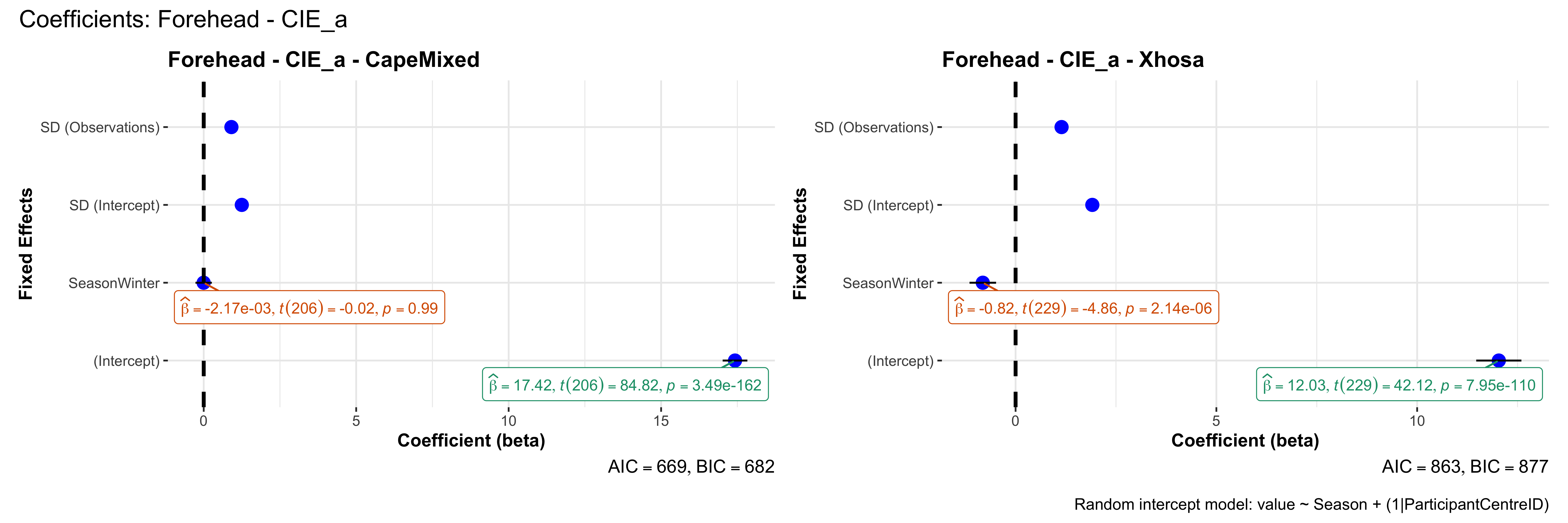
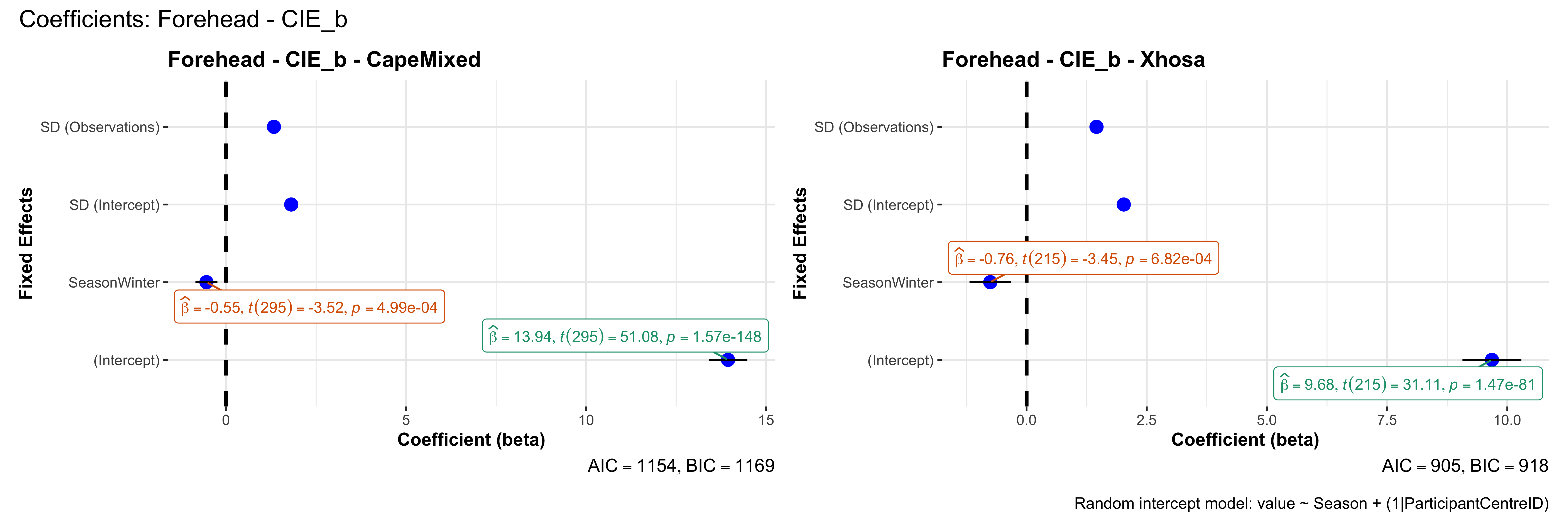
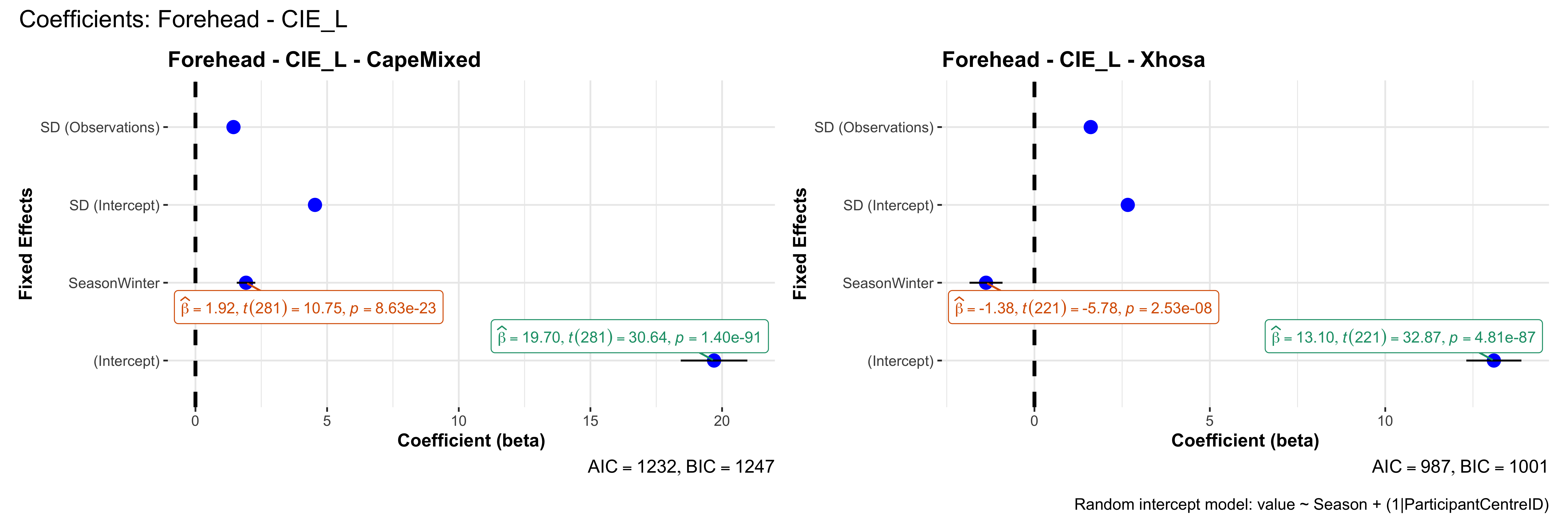
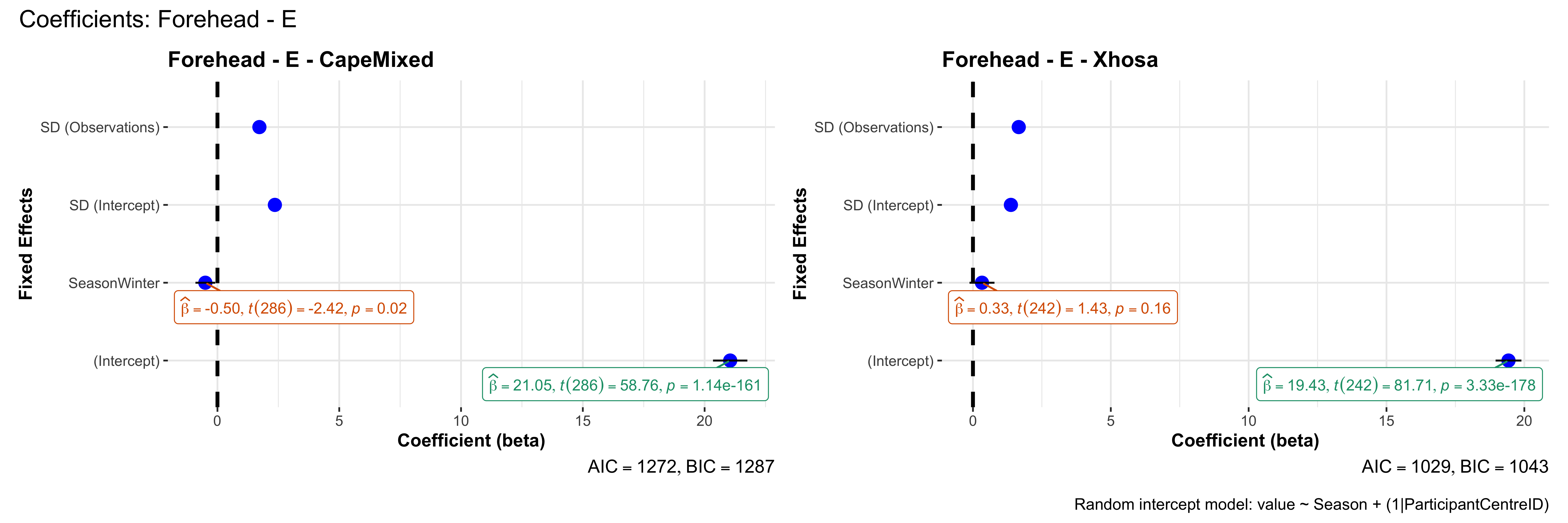
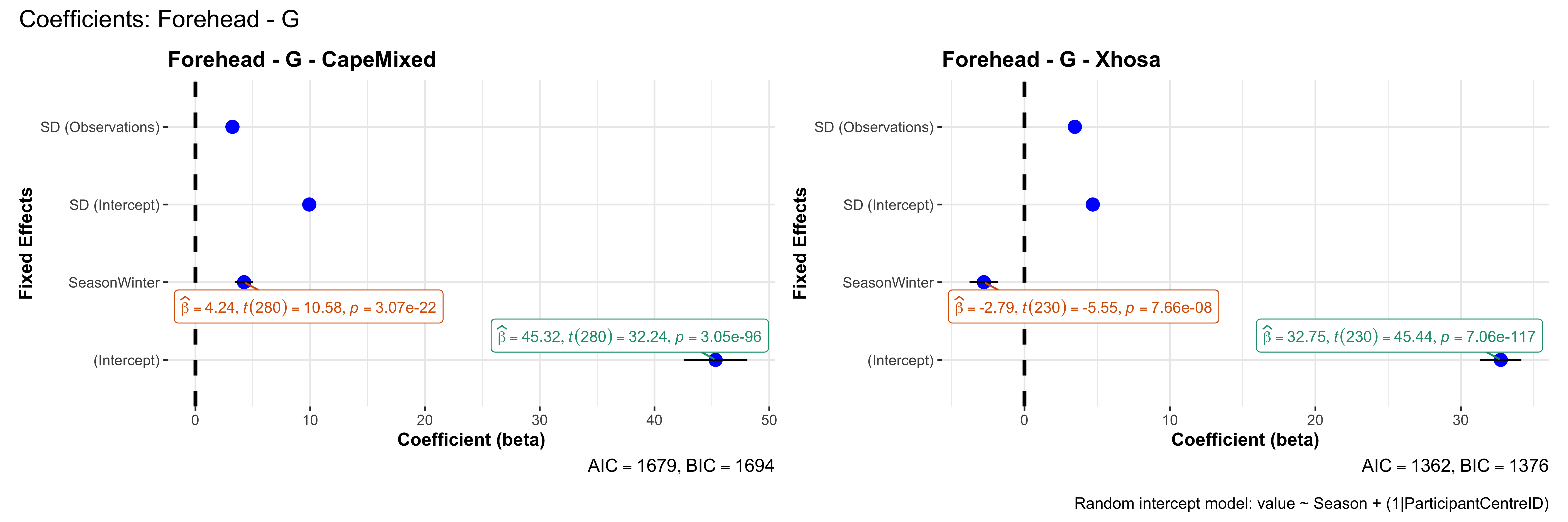
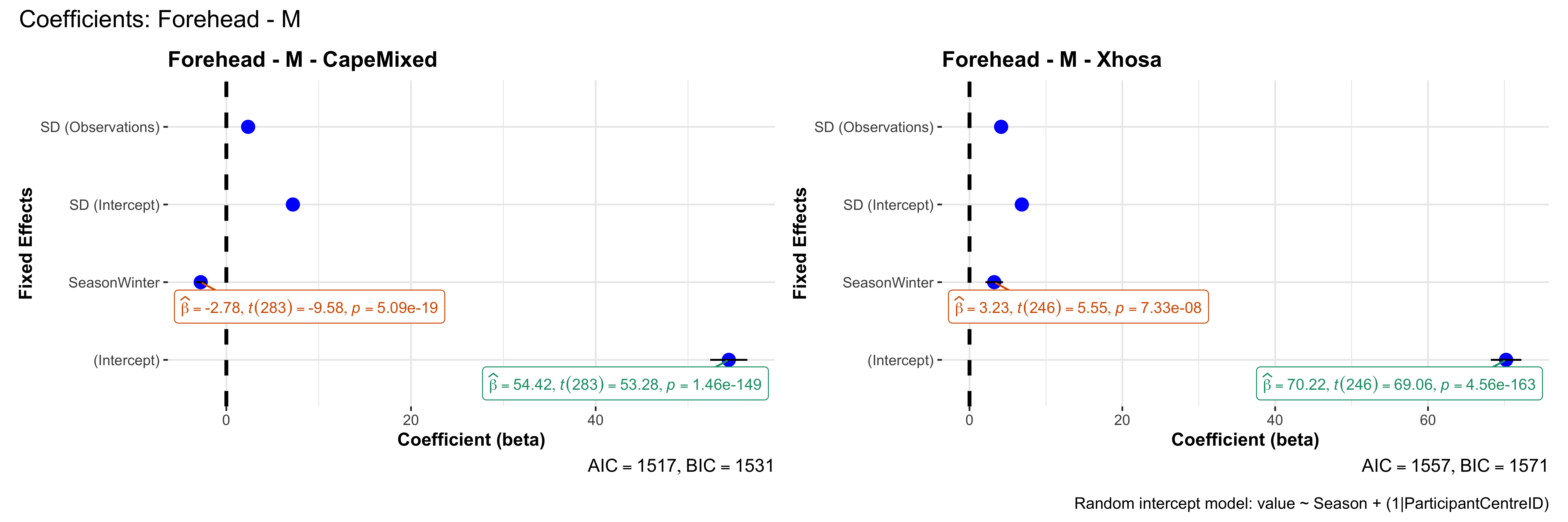
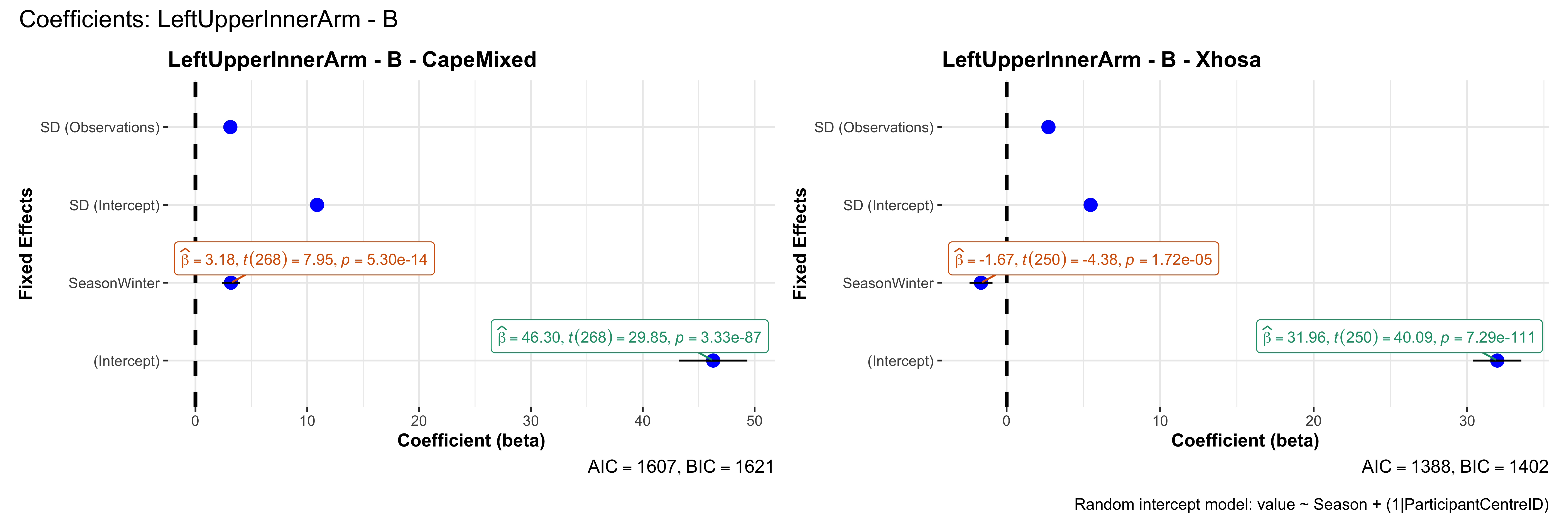
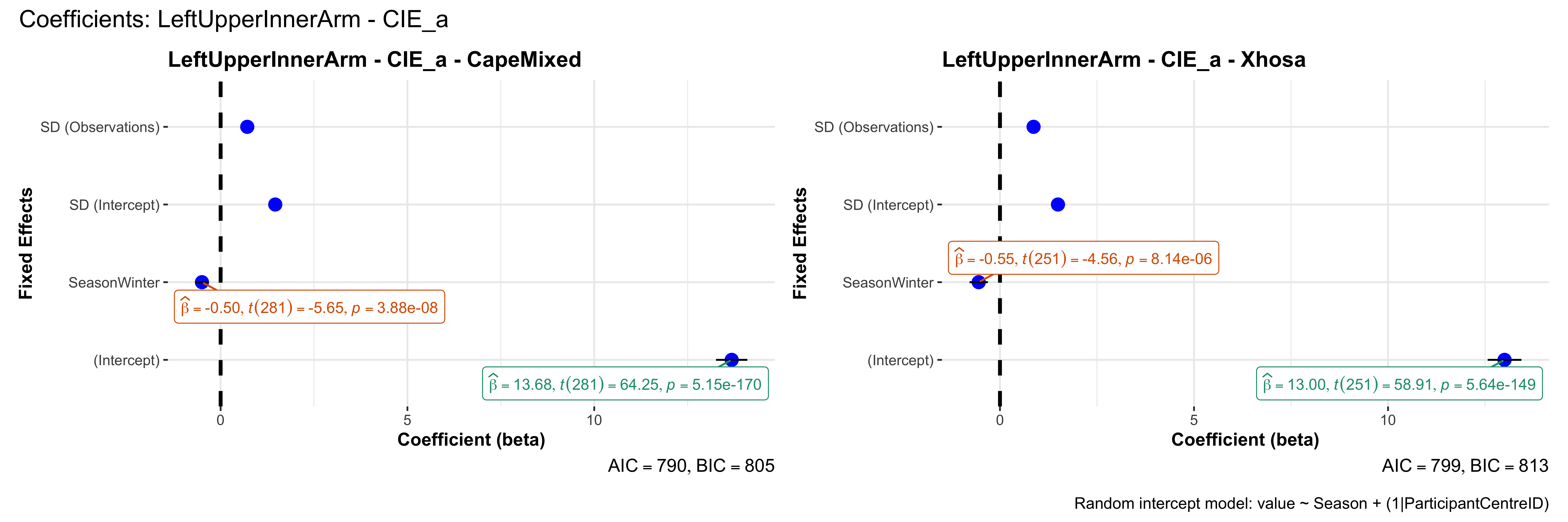
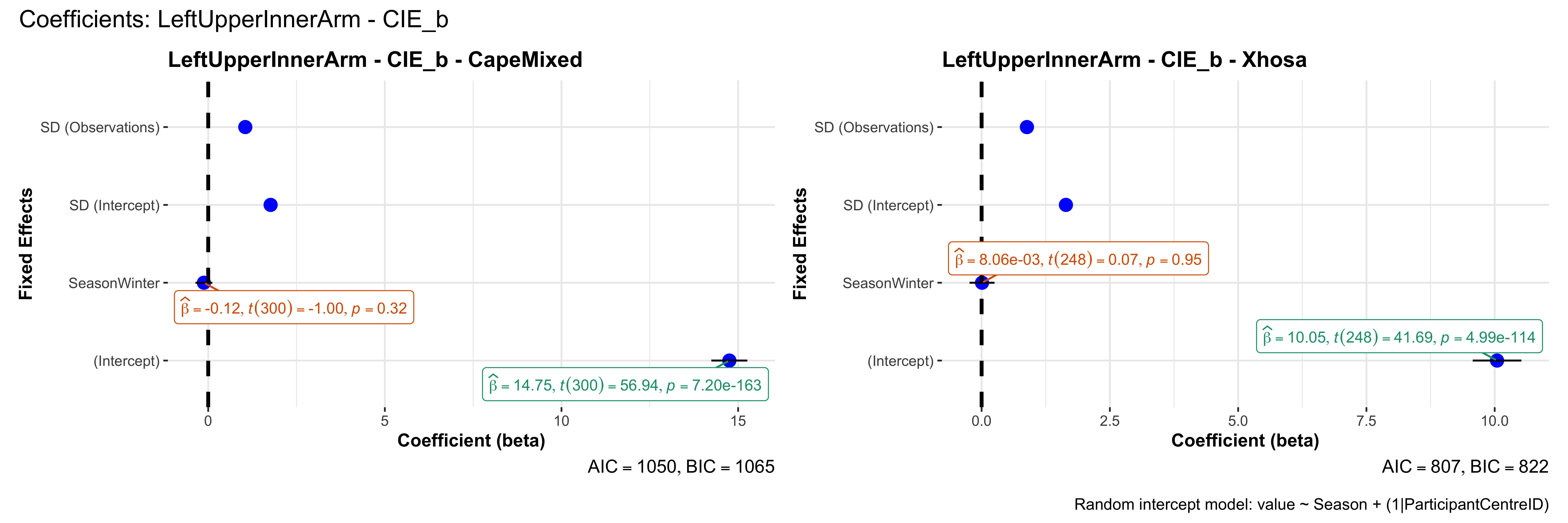
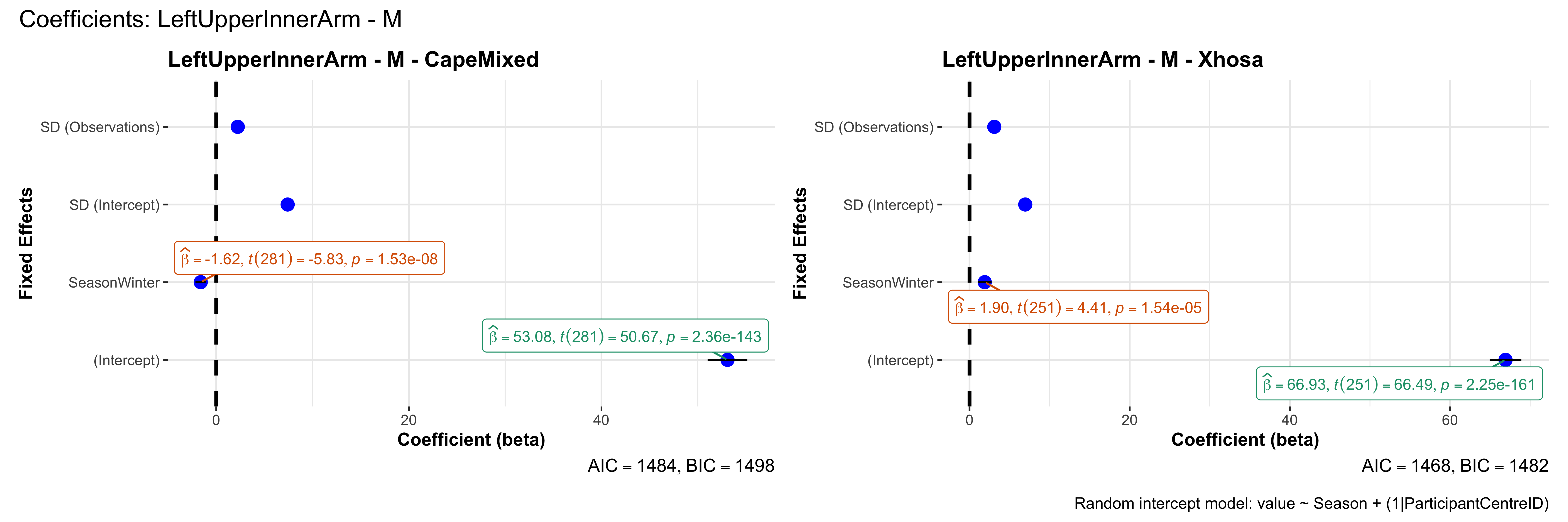
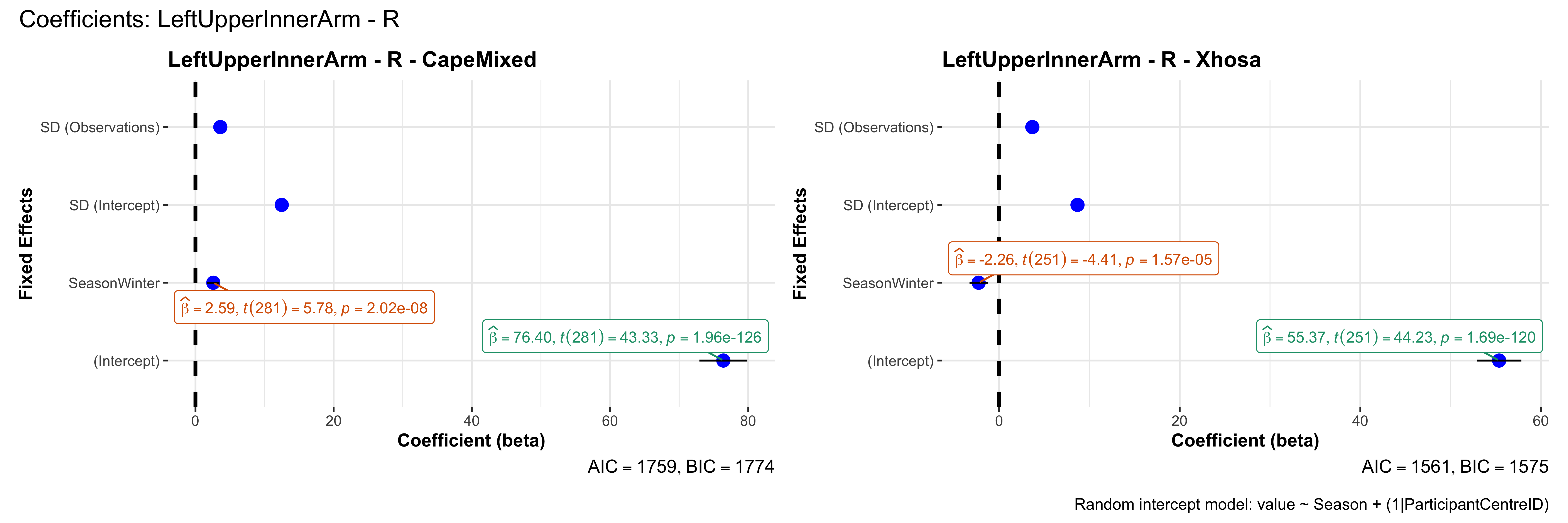
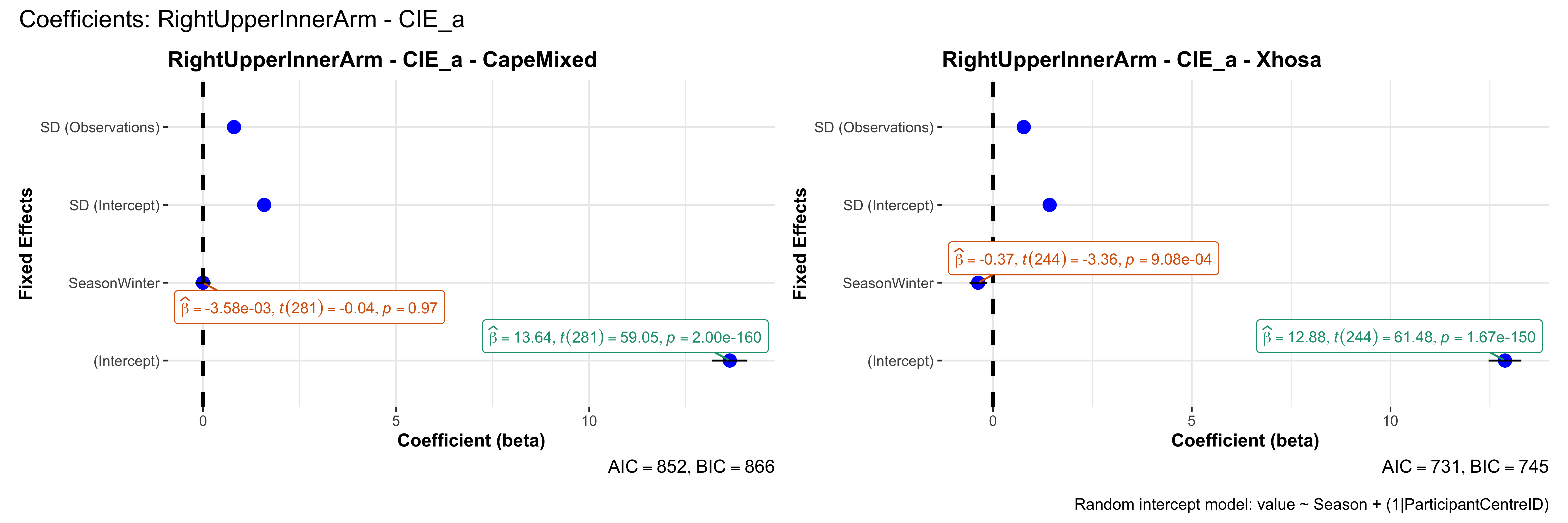
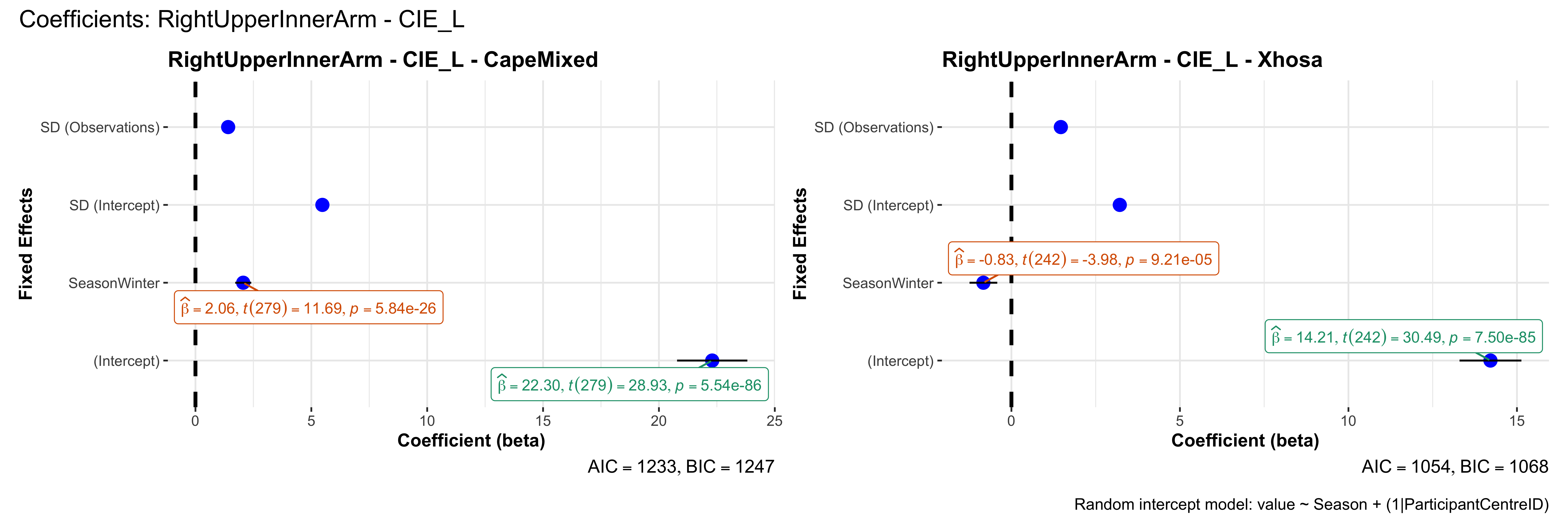
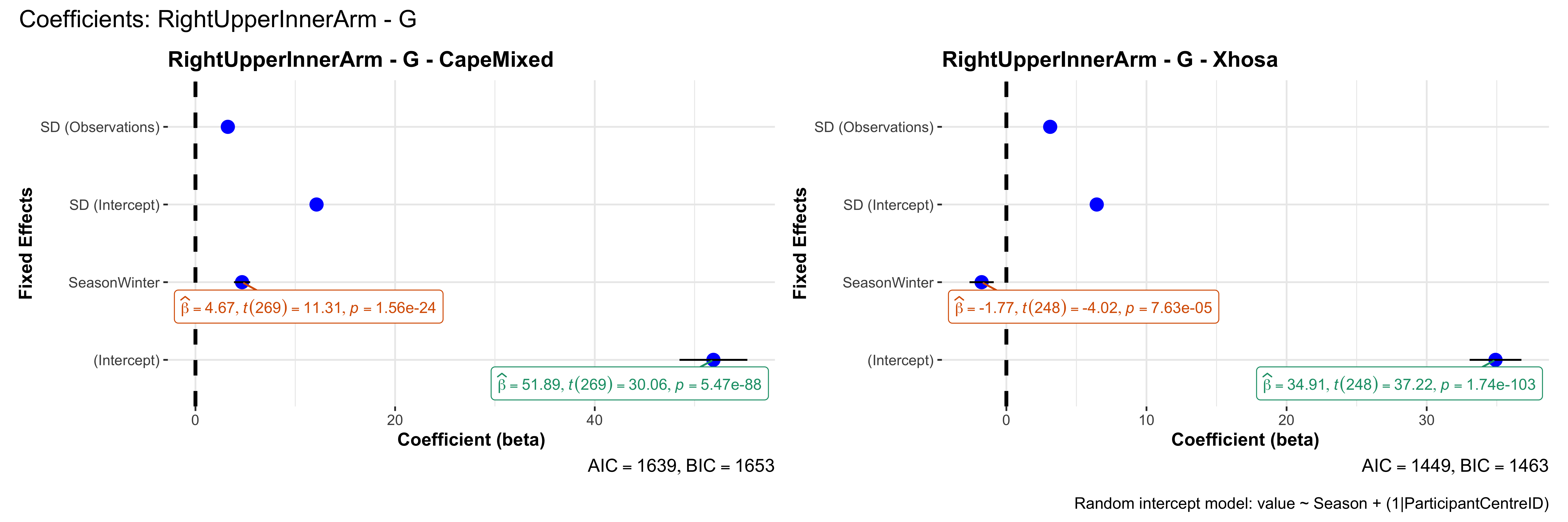
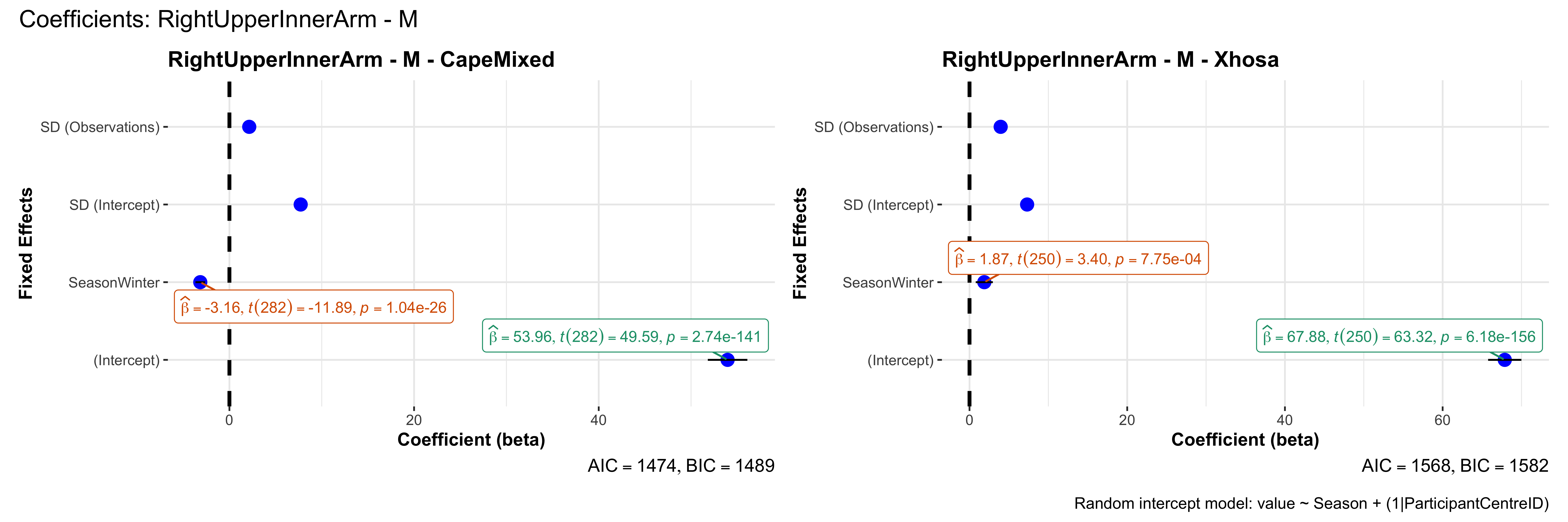
# in each subset.## ---- coeff-plots-summer-winter ----
## This script creates a single side-by-side (ncol=2) coefficient plot
## for each (body_site, measurement_type), comparing the two ethnic groups
## (e.g., "CapeMixed" vs. "Xhosa"). Each subplot shows a random-intercept
## model's coefficients for value ~ Season + (1|ParticipantCentreID).
library(lmerTest)
library(tidyverse)
library(ggstatsplot)
# 1) Load and clean your stage2_data
stage2_data <- read_csv("data/ScreeningDataCollection_stage2.csv") |>
group_by(ParticipantCentreID, body_site, measurement_type, Season) |>
mutate(
# Subtract however many NA values are in 'value' from n_valid
n_valid = n_valid - sum(is.na(value))
) |>
ungroup() |>
# Then remove rows with NA in 'value'
filter(!is.na(value)) |>
# Keep only Summer/Winter
filter(Season %in% c("Summer","Winter")) |>
mutate(
Season = factor(Season, levels=c("Summer","Winter")),
body_site = factor(body_site),
measurement_type = factor(measurement_type),
Ethnicity = factor(Ethnicity),
ParticipantCentreID= factor(ParticipantCentreID)
)
# 2) Identify combos of body_site + measurement_type
combos <- stage2_data |>
distinct(body_site, measurement_type) |>
arrange(body_site, measurement_type)
# 3) Create a directory "output/coeff_plots_summer-winter"
dir.create("output/coeff_plots_summer-winter", showWarnings = FALSE, recursive = TRUE)
# 4) We'll handle two ethnic groups side-by-side: "CapeMixed" & "Xhosa"
ethnic_groups <- c("CapeMixed", "Xhosa")
for (i in seq_len(nrow(combos))) {
bs <- combos$body_site[i]
mt <- combos$measurement_type[i]
# We'll store the two coefficient plots in a list
plot_list <- list()
valid_plots <- 0
for (eth in ethnic_groups) {
# Subset data
sub_data <- stage2_data |>
filter(body_site == bs, measurement_type == mt, Ethnicity == eth)
if (nrow(sub_data) < 4) {
message("Skipping: ", bs, " - ", mt, " - ", eth, " => not enough data.")
plot_list[[eth]] <- NULL
next
}
# Fit a random intercept model
mod <- tryCatch({
lmer(value ~ Season + (1|ParticipantCentreID), data=sub_data)
}, error = function(e) NULL)
if (is.null(mod)) {
message("Model failed for: ", bs, " - ", mt, " - ", eth)
plot_list[[eth]] <- NULL
next
}
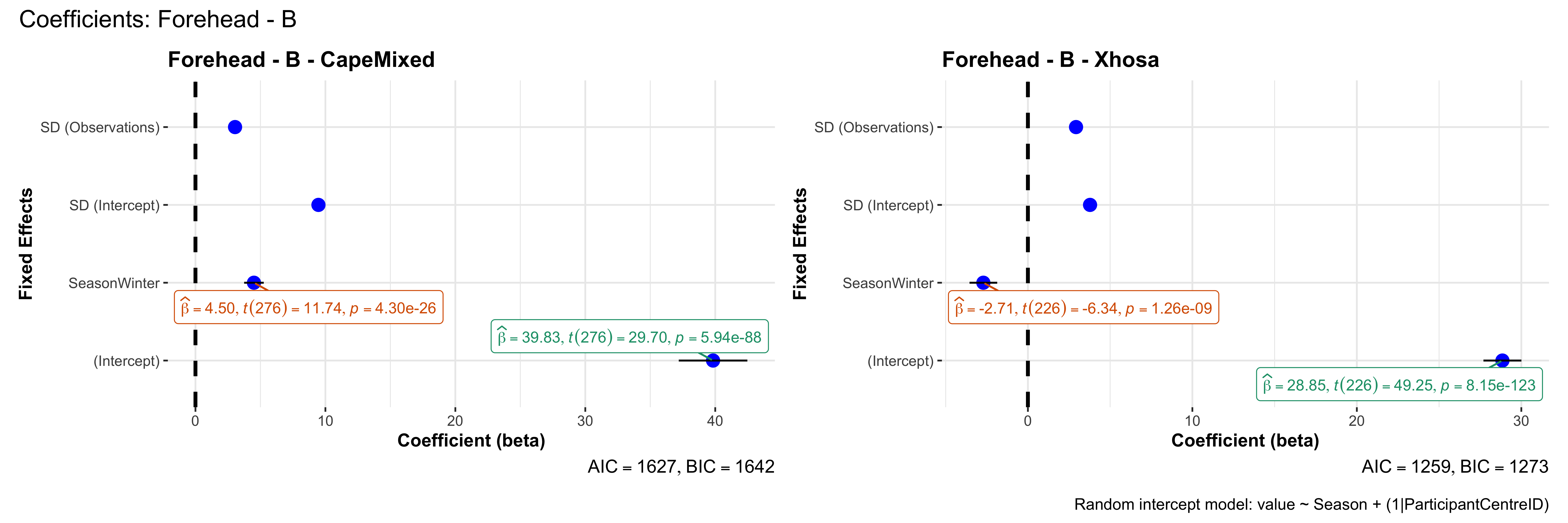
# Create a coefficient plot
plot_title <- paste0(bs, " - ", as.character(mt), " - ", eth)
p <- ggcoefstats(
x = mod,
title = plot_title,
xlab = "Coefficient (beta)",
ylab = "Fixed Effects"
)
plot_list[[eth]] <- p
valid_plots <- valid_plots + 1
}
# If neither ethnicity had enough data, skip saving
if (valid_plots == 0) {
next
}
# 5) Combine the two coefficient plots side by side (ncol=2)
# If one ethnicity was missing data, combine_plots can handle a NULL
final_plot <- combine_plots(
plotlist = plot_list,
plotgrid.args = list(ncol = 2),
annotation.args= list(
title = paste0("Coefficients: ", bs, " - ", mt),
caption = "Random intercept model: value ~ Season + (1|ParticipantCentreID)"
)
)
# 6) Save
outfile <- paste0("output/coeff_plots_summer-winter/coeff_", bs, "_", mt, ".png")
ggsave(outfile, final_plot, width=12, height=4)
# message("Saved: ", outfile)
# 7) **Print** to see in the knitted doc
print(final_plot)
}


sessionInfo()R version 4.4.3 (2025-02-28)
Platform: aarch64-apple-darwin20
Running under: macOS Sequoia 15.3.1
Matrix products: default
BLAS: /Library/Frameworks/R.framework/Versions/4.4-arm64/Resources/lib/libRblas.0.dylib
LAPACK: /Library/Frameworks/R.framework/Versions/4.4-arm64/Resources/lib/libRlapack.dylib; LAPACK version 3.12.0
locale:
[1] en_US.UTF-8/en_US.UTF-8/en_US.UTF-8/C/en_US.UTF-8/en_US.UTF-8
time zone: America/Detroit
tzcode source: internal
attached base packages:
[1] stats graphics grDevices utils datasets methods base
other attached packages:
[1] lmerTest_3.1-3 lme4_1.1-36 Matrix_1.7-2 lubridate_1.9.4
[5] forcats_1.0.0 stringr_1.5.1 dplyr_1.1.4 purrr_1.0.4
[9] readr_2.1.5 tidyr_1.3.1 tibble_3.2.1 ggplot2_3.5.1
[13] tidyverse_2.0.0 ggstatsplot_0.13.0 workflowr_1.7.1
loaded via a namespace (and not attached):
[1] Rdpack_2.6.2 pbapply_1.7-2 rematch2_2.1.2
[4] rlang_1.1.5 magrittr_2.0.3 git2r_0.35.0
[7] compiler_4.4.3 statsExpressions_1.6.2 getPass_0.2-4
[10] systemfonts_1.2.1 callr_3.7.6 vctrs_0.6.5
[13] pkgconfig_2.0.3 crayon_1.5.3 fastmap_1.2.0
[16] labeling_0.4.3 effectsize_1.0.0 promises_1.3.2
[19] rmarkdown_2.29 tzdb_0.4.0 ps_1.8.1
[22] nloptr_2.1.1 ragg_1.3.3 MatrixModels_0.5-3
[25] bit_4.5.0.1 xfun_0.50 cachem_1.1.0
[28] jsonlite_1.8.9 later_1.4.1 parallel_4.4.3
[31] R6_2.5.1 bslib_0.9.0 stringi_1.8.4
[34] boot_1.3-31 numDeriv_2016.8-1.1 jquerylib_0.1.4
[37] estimability_1.5.1 Rcpp_1.0.14 knitr_1.49
[40] parameters_0.24.2 correlation_0.8.7 httpuv_1.6.15
[43] splines_4.4.3 timechange_0.3.0 tidyselect_1.2.1
[46] rstudioapi_0.17.1 yaml_2.3.10 processx_3.8.5
[49] lattice_0.22-6 withr_3.0.2 bayestestR_0.15.2
[52] coda_0.19-4.1 evaluate_1.0.3 RcppParallel_5.1.10
[55] pillar_1.10.1 whisker_0.4.1 reformulas_0.4.0
[58] insight_1.1.0 generics_0.1.3 vroom_1.6.5
[61] rprojroot_2.0.4 paletteer_1.6.0 hms_1.1.3
[64] rstantools_2.4.0 munsell_0.5.1 scales_1.3.0
[67] minqa_1.2.8 glue_1.8.0 emmeans_1.10.7
[70] tools_4.4.3 fs_1.6.5 mvtnorm_1.3-3
[73] grid_4.4.3 rbibutils_2.3 datawizard_1.0.1
[76] colorspace_2.1-1 nlme_3.1-167 patchwork_1.3.0
[79] performance_0.13.0 cli_3.6.3 textshaping_1.0.0
[82] gtable_0.3.6 zeallot_0.1.0 sass_0.4.9
[85] digest_0.6.37 prismatic_1.1.2 ggrepel_0.9.6
[88] farver_2.1.2 htmltools_0.5.8.1 lifecycle_1.0.4
[91] httr_1.4.7 bit64_4.6.0-1 BayesFactor_0.9.12-4.7
[94] MASS_7.3-64