Lily Analysis
Lily Heald
2025-03-07
Last updated: 2025-04-11
Checks: 6 1
Knit directory: sapphire/
This reproducible R Markdown analysis was created with workflowr (version 1.7.1). The Checks tab describes the reproducibility checks that were applied when the results were created. The Past versions tab lists the development history.
Great! Since the R Markdown file has been committed to the Git repository, you know the exact version of the code that produced these results.
Great job! The global environment was empty. Objects defined in the global environment can affect the analysis in your R Markdown file in unknown ways. For reproduciblity it’s best to always run the code in an empty environment.
The command set.seed(20240923) was run prior to running
the code in the R Markdown file. Setting a seed ensures that any results
that rely on randomness, e.g. subsampling or permutations, are
reproducible.
Great job! Recording the operating system, R version, and package versions is critical for reproducibility.
Nice! There were no cached chunks for this analysis, so you can be confident that you successfully produced the results during this run.
Using absolute paths to the files within your workflowr project makes it difficult for you and others to run your code on a different machine. Change the absolute path(s) below to the suggested relative path(s) to make your code more reproducible.
| absolute | relative |
|---|---|
| ~/sapphire/SAfrADMIX/SAfrADMIX.ped | SAfrADMIX/SAfrADMIX.ped |
| ~/sapphire/SAfrADMIX/SAfrADMIX.map | SAfrADMIX/SAfrADMIX.map |
Great! You are using Git for version control. Tracking code development and connecting the code version to the results is critical for reproducibility.
The results in this page were generated with repository version e8fdf1b. See the Past versions tab to see a history of the changes made to the R Markdown and HTML files.
Note that you need to be careful to ensure that all relevant files for
the analysis have been committed to Git prior to generating the results
(you can use wflow_publish or
wflow_git_commit). workflowr only checks the R Markdown
file, but you know if there are other scripts or data files that it
depends on. Below is the status of the Git repository when the results
were generated:
Ignored files:
    Ignored:    .DS_Store
    Ignored:    .RData
    Ignored:    .Rhistory
    Ignored:    .Rproj.user/
    Ignored:    analysis/.RData
    Ignored:    analysis/.Rhistory
    Ignored:    data/.DS_Store
Note that any generated files, e.g. HTML, png, CSS, etc., are not included in this status report because it is ok for generated content to have uncommitted changes.
These are the previous versions of the repository in which changes were
made to the R Markdown (analysis/analysis1_PCAs.Rmd) and
HTML (docs/analysis1_PCAs.html) files. If you’ve configured
a remote Git repository (see ?wflow_git_remote), click on
the hyperlinks in the table below to view the files as they were in that
past version.
| File | Version | Author | Date | Message |
|---|---|---|---|---|
| Rmd | e8fdf1b | Lily Heald | 2025-04-11 | PC projections, UV data |
| Rmd | e86fbb5 | Lily Heald | 2025-04-04 | updated about cleaned redundant code |
| html | e86fbb5 | Lily Heald | 2025-04-04 | updated about cleaned redundant code |
| Rmd | 3fff1f9 | Lily Heald | 2025-04-04 | cleaning and climate data |
file_path <- "data/serum_vit_D_study_with_lab_results.xlsx"
data_summer <- read_excel(file_path, sheet = "ScreeningDataCollectionSummer")
data_winter <- read_excel(file_path, sheet = "ScreeningDataCollectionWinter")
data_6weeks <- read_excel(file_path, sheet = "ScreeningDataCollection6Weeks")
sun_expos <- read.csv("data/sun_expos_data/sun_expos_long.csv")
sun_expos_summer <- sun_expos[sun_expos$collection_period == 'Summer', ]
sun_expos_winter <- sun_expos[sun_expos$collection_period == 'Winter', ]
sun_expos_6Weeks <- sun_expos[sun_expos$collection_period == '6Weeks', ]
# SAfrADMIX <- read.table("~/sapphire/SAfrADMIX/SAfrADMIX.ped")
# SAfrADMIXm <- read.table("~/sapphire/SAfrADMIX/SAfrADMIX.map")
part 0: cleaning
summer_data <- left_join(data_summer, sun_expos_summer,
                     by = c("ParticipantCentreID" = "participant_centre_id"))

winter_data <- left_join(data_winter, sun_expos_winter,
                     by = c("ParticipantCentreID" = "participant_centre_id"))

six_week_data <- left_join(data_6weeks, sun_expos_6Weeks,
                     by = c("ParticipantCentreID" = "participant_centre_id"))
summer_data = subset(summer_data, select = -c(Supplements, Medications,
EthnicitySpecifyOther, SmokingComments,
x9if_apply_sunscreen_spf_used))
winter_data = subset(winter_data, select = -c(Supplements, Medications,
EthnicitySpecifyOther, SmokingComments,
ContinuedInStudy, IfNotContinuedInStudyReason,
x9if_apply_sunscreen_spf_used))
six_week_data = subset(six_week_data, select = -c(Supplements, Medications,
EthnicitySpecifyOther, SmokingComments,
ContinuedInStudy, IfNotContinuedInStudyReason,
x9if_apply_sunscreen_spf_used))
six_week_data = six_week_data[,!grepl("IfNoReasonForExclusion:",names(six_week_data))]
winter_data = winter_data[,!grepl("IfNoReasonForExclusion:",names(winter_data))]
summer_data = summer_data[,!grepl("IfNoReasonForExclusion:",names(summer_data))]
six_week_data = six_week_data[,!grepl("Req Num",names(six_week_data))]
winter_data = winter_data[,!grepl("Req Num",names(winter_data))]
summer_data = summer_data[,!grepl("Req Num",names(summer_data))]# taking the median of three measurements
sites <- c("Forehead", "RightUpperInnerArm", "LeftUpperInnerArm")
metrics <- c("E", "M", "R", "G", "B", "L\\*", "a\\*", "b\\*")
seasons <- c("six_week_data", "summer_data", "winter_data")
for(site in sites) {
for(metric in metrics) {
six_week_data <- six_week_data %>%
rowwise() %>%
mutate(!!paste0("Median", site, metric) := median(c_across(matches(paste0("SkinReflectance", site, metric, "[123]"))), na.rm = TRUE)) %>%
ungroup()
}
}
for(site in sites) {
for(metric in metrics) {
summer_data <- summer_data %>%
rowwise() %>%
mutate(!!paste0("Median", site, metric) := median(c_across(matches(paste0("SkinReflectance", site, metric, "[123]"))), na.rm = TRUE)) %>%
ungroup()
}
}
for(site in sites) {
for(metric in metrics) {
winter_data <- winter_data %>%
rowwise() %>%
mutate(!!paste0("Median", site, metric) := median(c_across(matches(paste0("SkinReflectance", site, metric, "[123]"))), na.rm = TRUE)) %>%
ungroup()
}
}
winter_data <- winter_data %>%
select(-matches(".*[EMRGBL\\*a\\*b\\*]\\d$"))
summer_data <- summer_data %>%
select(-matches(".*[EMRGBL\\*a\\*b\\*]\\d$"))
six_week_data <- six_week_data %>%
select(-matches(".*[EMRGBL\\*a\\*b\\*]\\d$"))ethnicity <- function(EthnicityAfricanBlack, EthnicityColoured, EthnicityWhite,
EthnicityIndianAsian) {
case_when(
EthnicityAfricanBlack == TRUE &
EthnicityColoured == FALSE &
EthnicityWhite == FALSE &
EthnicityIndianAsian == FALSE ~ "Xhosa",
EthnicityAfricanBlack == FALSE &
EthnicityColoured == TRUE &
EthnicityWhite == FALSE &
EthnicityIndianAsian == FALSE ~ "Cape_colored",
TRUE ~ NA_character_
)
}
summer_data <- summer_data %>%
mutate(Ethnicity = ethnicity(EthnicityAfricanBlack, EthnicityColoured,
EthnicityWhite, EthnicityIndianAsian))
summer_data = subset(summer_data, select = -c(EthnicityAfricanBlack,
EthnicityColoured, EthnicityWhite,
EthnicityIndianAsian))
winter_data <- winter_data %>%
mutate(Ethnicity = ethnicity(EthnicityAfricanBlack, EthnicityColoured,
EthnicityWhite, EthnicityIndianAsian))
winter_data = subset(winter_data, select = -c(EthnicityAfricanBlack,
EthnicityColoured, EthnicityWhite,
EthnicityIndianAsian))
six_week_data <- six_week_data %>%
mutate(Ethnicity = ethnicity(EthnicityAfricanBlack, EthnicityColoured,
EthnicityWhite, EthnicityIndianAsian))
six_week_data = subset(six_week_data, select = -c(EthnicityAfricanBlack,
EthnicityColoured, EthnicityWhite,
EthnicityIndianAsian))# mean left and right inner arm
for (metric in metrics) {
summer_data <- summer_data %>%
mutate(!!paste0("MedianInnerArm", metric) := rowMeans(
select(., starts_with(paste0("MedianLeftInnerArm", metric)),
starts_with(paste0("MedianRightUpperInnerArm", metric))),
na.rm = TRUE
))
}
for (metric in metrics) {
winter_data <- winter_data %>%
mutate(!!paste0("MedianInnerArm", metric) := rowMeans(
select(., starts_with(paste0("MedianLeftInnerArm", metric)),
starts_with(paste0("MedianRightUpperInnerArm", metric))),
na.rm = TRUE
))
}
for (metric in metrics) {
six_week_data <- six_week_data %>%
mutate(!!paste0("MedianInnerArm", metric) := rowMeans(
select(., starts_with(paste0("MedianLeftInnerArm", metric)),
starts_with(paste0("MedianRightUpperInnerArm", metric))),
na.rm = TRUE
))
}
winter_data <- winter_data %>%
select(-matches("Left|Right"))
summer_data <- summer_data %>%
select(-matches("Left|Right"))
six_week_data <- six_week_data %>%
select(-matches("Left|Right"))for (metric in metrics) {
six_week_data <- six_week_data %>%
mutate(!!paste0(metric, "Difference") :=
.[[paste0("MedianForehead", metric)]] -
.[[paste0("MedianInnerArm", metric)]])
}
for (metric in metrics) {
summer_data <- summer_data %>%
mutate(!!paste0(metric, "Difference") :=
.[[paste0("MedianForehead", metric)]] -
.[[paste0("MedianInnerArm", metric)]])
}
for (metric in metrics) {
winter_data <- winter_data %>%
mutate(!!paste0(metric, "Difference") :=
.[[paste0("MedianForehead", metric)]] -
.[[paste0("MedianInnerArm", metric)]])
}ggplot(six_week_data, aes(x = VitDResult, y = MedianForeheadM, color = Ethnicity)) +
geom_jitter() +
theme(legend.position = "right")Warning: Removed 1 row containing missing values or values outside the scale range
(`geom_point()`).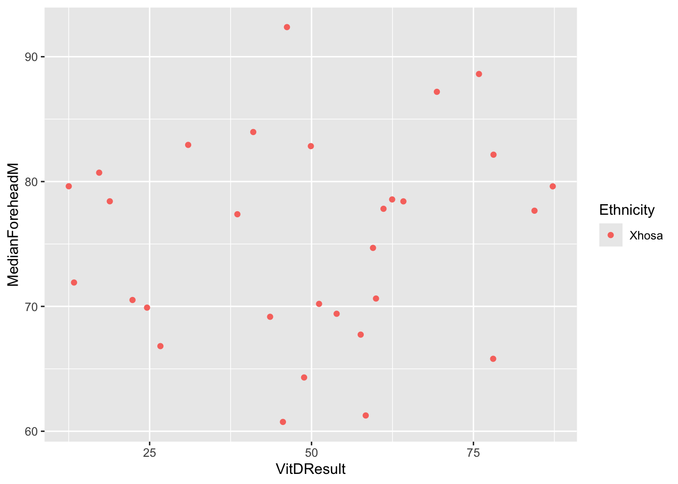
| Version | Author | Date |
|---|---|---|
| e86fbb5 | Lily Heald | 2025-04-04 |
ggplot(six_week_data, aes(x = Ethnicity, y = MedianForeheadM, color = Ethnicity, fill = Ethnicity)) +
  geom_violin()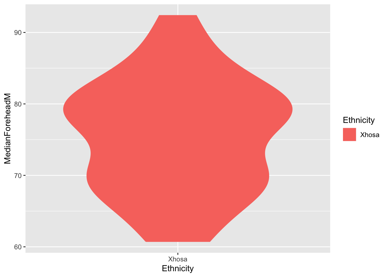
| Version | Author | Date |
|---|---|---|
| e86fbb5 | Lily Heald | 2025-04-04 |
ggplot(summer_data, aes(x = VitDResult, y = MedianForeheadM, color = Ethnicity)) +
  geom_jitter() +
  theme(legend.position = "right")
Warning: Removed 1 row containing missing values or values outside the scale range
(`geom_point()`).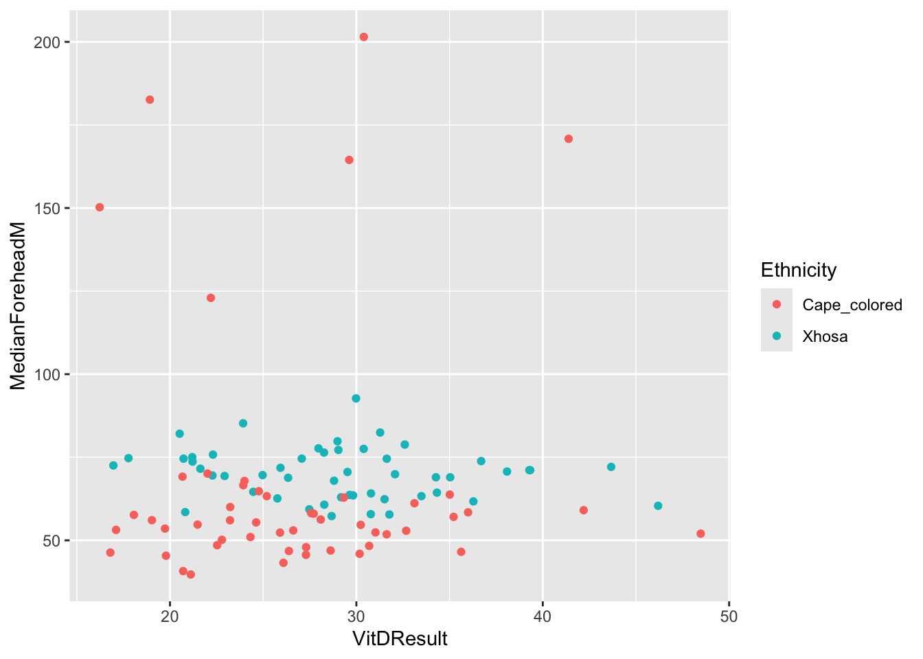
| Version | Author | Date |
|---|---|---|
| e86fbb5 | Lily Heald | 2025-04-04 |
ggplot(summer_data, aes(x = Ethnicity, y = MedianForeheadM, color = Ethnicity, fill = Ethnicity)) +
  geom_boxplot()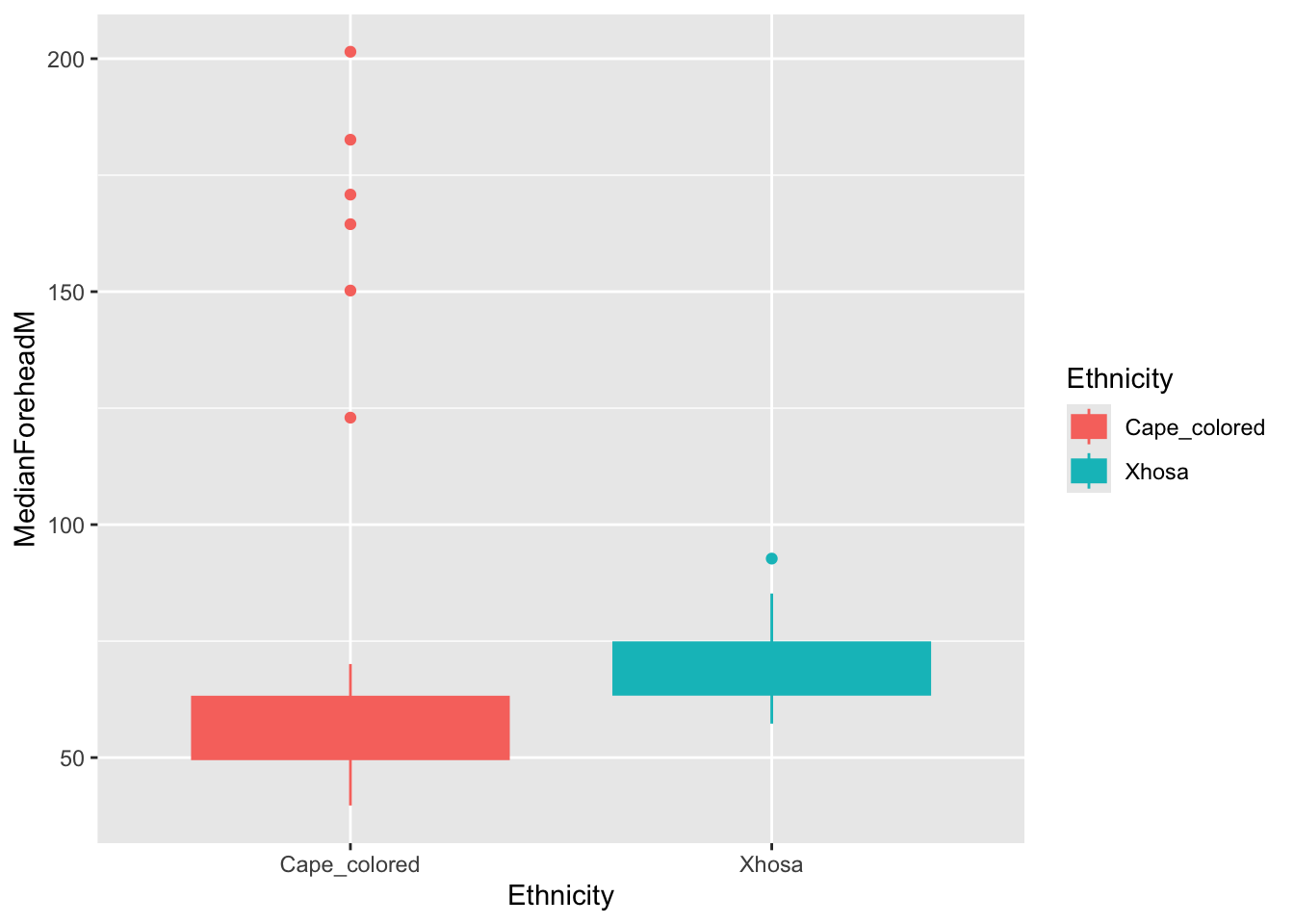
| Version | Author | Date |
|---|---|---|
| e86fbb5 | Lily Heald | 2025-04-04 |
# there are still outliers even when taking the median
sites <- c("Forehead", "InnerArm")
for(site in sites) {
  for(metric in metrics) {
    column_name <- paste0("Median", site, metric)
    iqr <- IQR(winter_data[[column_name]], na.rm = TRUE)
    Q <- quantile(winter_data[[column_name]], probs = c(0.25, 0.75), na.rm = TRUE)
    up <- Q[2] + 1.5 * iqr
    low <- Q[1] - 1.5 * iqr
    winter_data <- winter_data %>%
      filter(!!sym(column_name) > low & !!sym(column_name) < up)
  }
}

for(site in sites) {
  for(metric in metrics) {
    column_name <- paste0("Median", site, metric)
    iqr <- IQR(summer_data[[column_name]], na.rm = TRUE)
    Q <- quantile(summer_data[[column_name]], probs = c(0.25, 0.75), na.rm = TRUE)
    up <- Q[2] + 1.5 * iqr
    low <- Q[1] - 1.5 * iqr
    summer_data <- summer_data %>%
      filter(!!sym(column_name) > low & !!sym(column_name) < up)
  }
}

for(site in sites) {
  for(metric in metrics) {
    column_name <- paste0("Median", site, metric)
    iqr <- IQR(winter_data[[column_name]], na.rm = TRUE)
    Q <- quantile(winter_data[[column_name]], probs = c(0.25, 0.75), na.rm = TRUE)
    up <- Q[2] + 1.5 * iqr
    low <- Q[1] - 1.5 * iqr
    six_week_data <- six_week_data %>%
      filter(!!sym(column_name) > low & !!sym(column_name) < up)
  }
}
ggplot(six_week_data, aes(x = VitDResult, y = MedianForeheadM, color = Ethnicity)) +
geom_jitter() +
theme(legend.position = "right")Warning: Removed 1 row containing missing values or values outside the scale range
(`geom_point()`).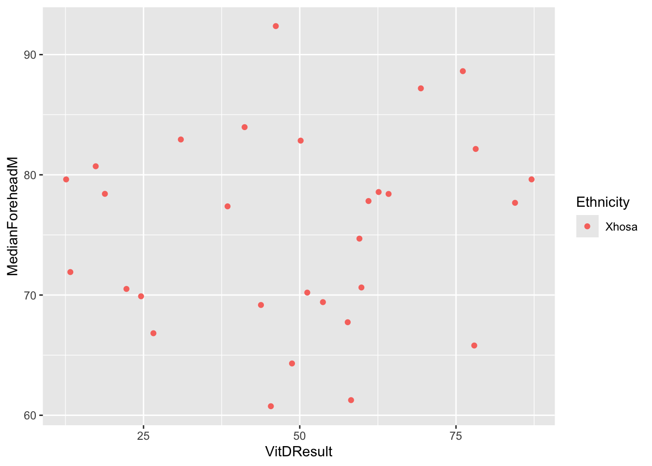
| Version | Author | Date |
|---|---|---|
| e86fbb5 | Lily Heald | 2025-04-04 |
ggplot(six_week_data, aes(x = Ethnicity, y = MedianForeheadM, color = Ethnicity, fill = Ethnicity)) +
  geom_violin()
| Version | Author | Date |
|---|---|---|
| e86fbb5 | Lily Heald | 2025-04-04 |
ggplot(summer_data, aes(x = VitDResult, y = MedianForeheadM, color = Ethnicity)) +
  geom_jitter() +
  theme(legend.position = "right")
Warning: Removed 1 row containing missing values or values outside the scale range
(`geom_point()`).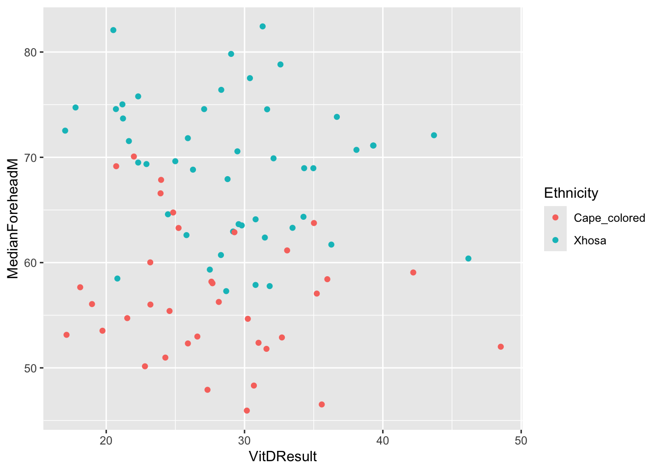
| Version | Author | Date |
|---|---|---|
| e86fbb5 | Lily Heald | 2025-04-04 |
ggplot(summer_data, aes(x = Ethnicity, y = MedianForeheadM, color = Ethnicity, fill = Ethnicity)) +
  geom_boxplot()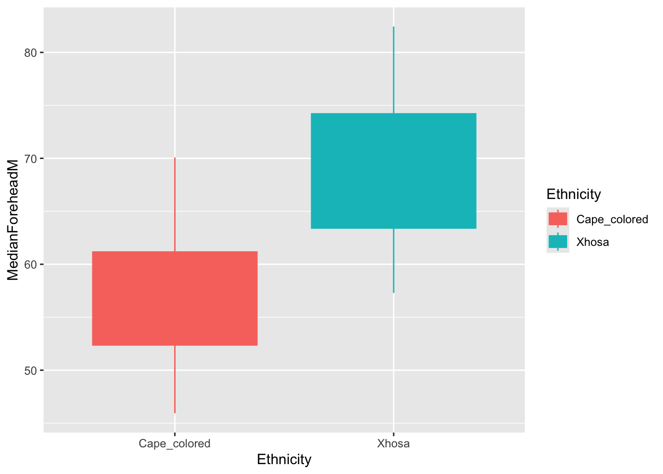
| Version | Author | Date |
|---|---|---|
| e86fbb5 | Lily Heald | 2025-04-04 |
six_week_rename <- six_week_data %>%
    rename_with(~ paste0(., "-6weeks"), -ParticipantCentreID)

joinone <- left_join(summer_data, winter_data,
                     by = "ParticipantCentreID",
                     suffix = c("-summer", "-winter"))

joined_data <- left_join(joinone, six_week_rename,
                         by = "ParticipantCentreID")

head(joined_data)
# A tibble: 6 × 256
ParticipantCentreID `InterviewerName-summer` `TodayDate-summer`
<chr> <chr> <dttm>
1 VDKH001 Betty 2013-02-11 00:00:00
2 VDKH002 Betty 2013-02-11 00:00:00
3 VDKH003 Betty 2013-02-11 00:00:00
4 VDKH004 Betty 2013-02-12 00:00:00
5 VDKH005 Betty 2013-02-12 00:00:00
6 VDKH006 Betty 2013-02-12 00:00:00
# ℹ 253 more variables: `AgeYears-summer` <dbl>, `DateOfBirth-summer` <dttm>,
# `Gender-summer` <dbl>, `EthnicityOther-summer` <lgl>,
# `Ethnicity-summer` <chr>, `RefuseToAnswer-summer` <lgl>,
# `AvgWeight-summer` <dbl>, `AvgHeight-summer` <dbl>, `BMI-summer` <dbl>,
# `SoreThroatYes-summer` <lgl>, `SoreThroatNo-summer` <lgl>,
# `RunnyNoseYes-summer` <lgl>, `RunnyNoseNo-summer` <lgl>,
# `CoughYes-summer` <lgl>, `CoughNo-summer` <lgl>, `FeverYes-summer` <lgl>, …#join into pheno_dat
six_week_rename <- six_week_data %>%
rename_with(~ paste0(., "-6weeks"), -ParticipantCentreID)
phenojoinone <- left_join(summer_data, winter_data,
by = "ParticipantCentreID",
suffix = c("-summer", "-winter"))
pheno_dat <- left_join(phenojoinone, six_week_rename,
by = "ParticipantCentreID")
# create tanning columns
pheno_dat <- pheno_dat %>%
mutate(tanning = coalesce(`MDifference-summer` - `MDifference-winter`, 0),
foreheadtanning = coalesce(`MedianForeheadM-summer` - `MedianForeheadM-winter`, 0))
#change ParticipantCentreID to IID
pheno_dat$ParticipantCentreID <- gsub("([A-Z]{4})0([0-9]{2})", "\\1\\2", pheno_dat$ParticipantCentreID)
names(pheno_dat)[names(pheno_dat) == "ParticipantCentreID"] <- "IID"
pheno_dat$IID <- gsub("VDKH([0-9]+)", "VDKHS\\1", pheno_dat$IID)
#subset by phenotype data
pheno_dat <- pheno_dat %>%
select(matches("MedianForehead|InnerArm|Difference|tanning|VitD|IID"))
#Create FID
pheno_dat <- pheno_dat %>%
mutate(FID = case_when(
grepl("^VDTG", IID) ~ gsub("^VDTG", "CM", IID),
grepl("^VDKHS", IID) ~ gsub("^VDKHS", "XH", IID),
TRUE ~ IID))
# move FID to first column to match format
pheno_dat <- pheno_dat %>%
select("FID", everything())
tanning_data <- pheno_dat %>%
select(c("FID", "IID", "foreheadtanning"))part 1: PCAs
PCAs to run: - run wideform pca - run pigmentation subset pca for each season - run RGB subset for each season - run ME subset for each season - run CIElab subset for each season
wideform
summer_winter <- left_join(summer_data, winter_data,
                     by = "ParticipantCentreID",
                     suffix = c("-summer", "-winter"))
summer_winter_clean <- na.omit(summer_winter)
reflectance_metrics_ws <- summer_winter_clean %>%
select(matches("MedianForehead|InnerArm"))
reflectance_metrics_ws# A tibble: 62 × 32
`MedianForeheadE-summer` `MedianForeheadM-summer` `MedianForeheadR-summer`
<dbl> <dbl> <dbl>
1 18.6 70.6 50
2 17.4 74.7 45
3 14.3 69.6 51
4 19.7 63.0 57
5 15.3 82.1 38
6 23.8 69.0 51
7 18.9 59.3 66
8 18.6 64.6 59
9 18.3 79.8 39
10 15.5 75.0 44
# ℹ 52 more rows
# ℹ 29 more variables: `MedianForeheadG-summer` <dbl>,
# `MedianForeheadB-summer` <dbl>, `MedianForeheadL\\*-summer` <dbl>,
# `MedianForeheada\\*-summer` <dbl>, `MedianForeheadb\\*-summer` <dbl>,
# `MedianInnerArmE-summer` <dbl>, `MedianInnerArmM-summer` <dbl>,
# `MedianInnerArmR-summer` <dbl>, `MedianInnerArmG-summer` <dbl>,
# `MedianInnerArmB-summer` <dbl>, `MedianInnerArmL\\*-summer` <dbl>, …reflectance3 <- scale(reflectance_metrics_ws)
reflectancepcaws <- prcomp(reflectance3)
summary(reflectancepcaws)Importance of components:
PC1 PC2 PC3 PC4 PC5 PC6 PC7
Standard deviation 4.8708 1.76349 1.30313 0.98821 0.75880 0.72092 0.68732
Proportion of Variance 0.7414 0.09718 0.05307 0.03052 0.01799 0.01624 0.01476
Cumulative Proportion 0.7414 0.83857 0.89163 0.92215 0.94014 0.95639 0.97115
PC8 PC9 PC10 PC11 PC12 PC13 PC14
Standard deviation 0.53700 0.44642 0.39456 0.27647 0.21339 0.18908 0.16793
Proportion of Variance 0.00901 0.00623 0.00486 0.00239 0.00142 0.00112 0.00088
Cumulative Proportion 0.98016 0.98639 0.99125 0.99364 0.99506 0.99618 0.99706
PC15 PC16 PC17 PC18 PC19 PC20 PC21
Standard deviation 0.15503 0.13513 0.11606 0.09057 0.08605 0.07618 0.06043
Proportion of Variance 0.00075 0.00057 0.00042 0.00026 0.00023 0.00018 0.00011
Cumulative Proportion 0.99781 0.99838 0.99881 0.99906 0.99929 0.99947 0.99959
PC22 PC23 PC24 PC25 PC26 PC27 PC28
Standard deviation 0.0575 0.04986 0.04625 0.03954 0.03070 0.02852 0.02518
Proportion of Variance 0.0001 0.00008 0.00007 0.00005 0.00003 0.00003 0.00002
Cumulative Proportion 0.9997 0.99977 0.99984 0.99989 0.99991 0.99994 0.99996
PC29 PC30 PC31 PC32
Standard deviation 0.02232 0.01997 0.01714 0.009283
Proportion of Variance 0.00002 0.00001 0.00001 0.000000
Cumulative Proportion 0.99998 0.99999 1.00000 1.000000reflectancepcaws$loadings[, 1:2]NULLfviz_eig(reflectancepcaws, addlabels = TRUE)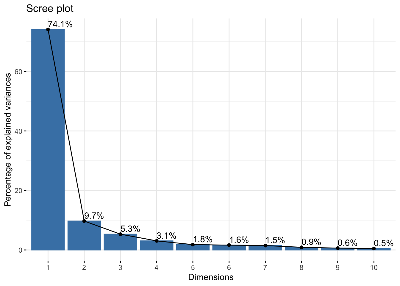
| Version | Author | Date |
|---|---|---|
| e86fbb5 | Lily Heald | 2025-04-04 |
fviz_pca_var(reflectancepcaws, col.var = "black")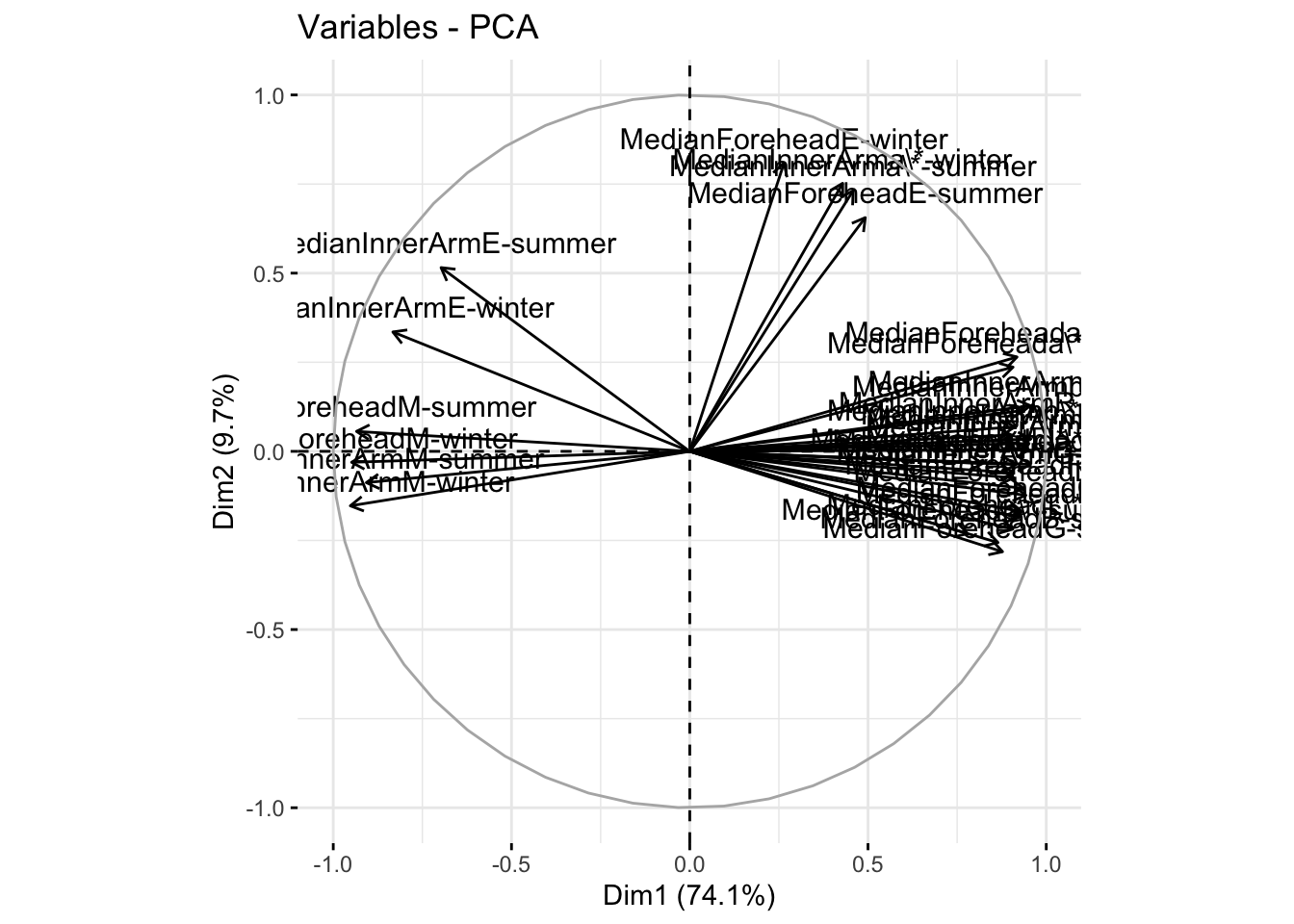
| Version | Author | Date |
|---|---|---|
| e86fbb5 | Lily Heald | 2025-04-04 |
fviz_cos2(reflectancepcaws, choice = "var", axes = 1:2)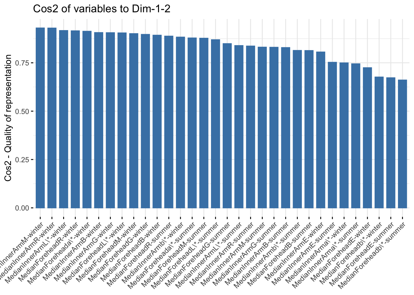
| Version | Author | Date |
|---|---|---|
| e86fbb5 | Lily Heald | 2025-04-04 |
wscomps <- as.data.frame(reflectancepcaws$x)
reflectance_ws <- cbind(summer_winter_clean,wscomps[,c(1,2)])
reflectance_ws <- reflectance_ws %>%
  select(-matches("SkinReflectance"))
reflectance_ws <- reflectance_ws %>%
  select(-"Ethnicity-winter")
names(reflectance_ws)[names(reflectance_ws) == 'Ethnicity-summer'] <- 'Ethnicity'


ggplot(reflectance_ws, aes(x=PC1, y=PC2, col = Ethnicity, fill = Ethnicity)) +
  stat_ellipse(geom = "polygon", col= "black", alpha =0.5)+
  geom_point(shape=21, col="black") +
  labs(title = "Wide Pigmentation PCA")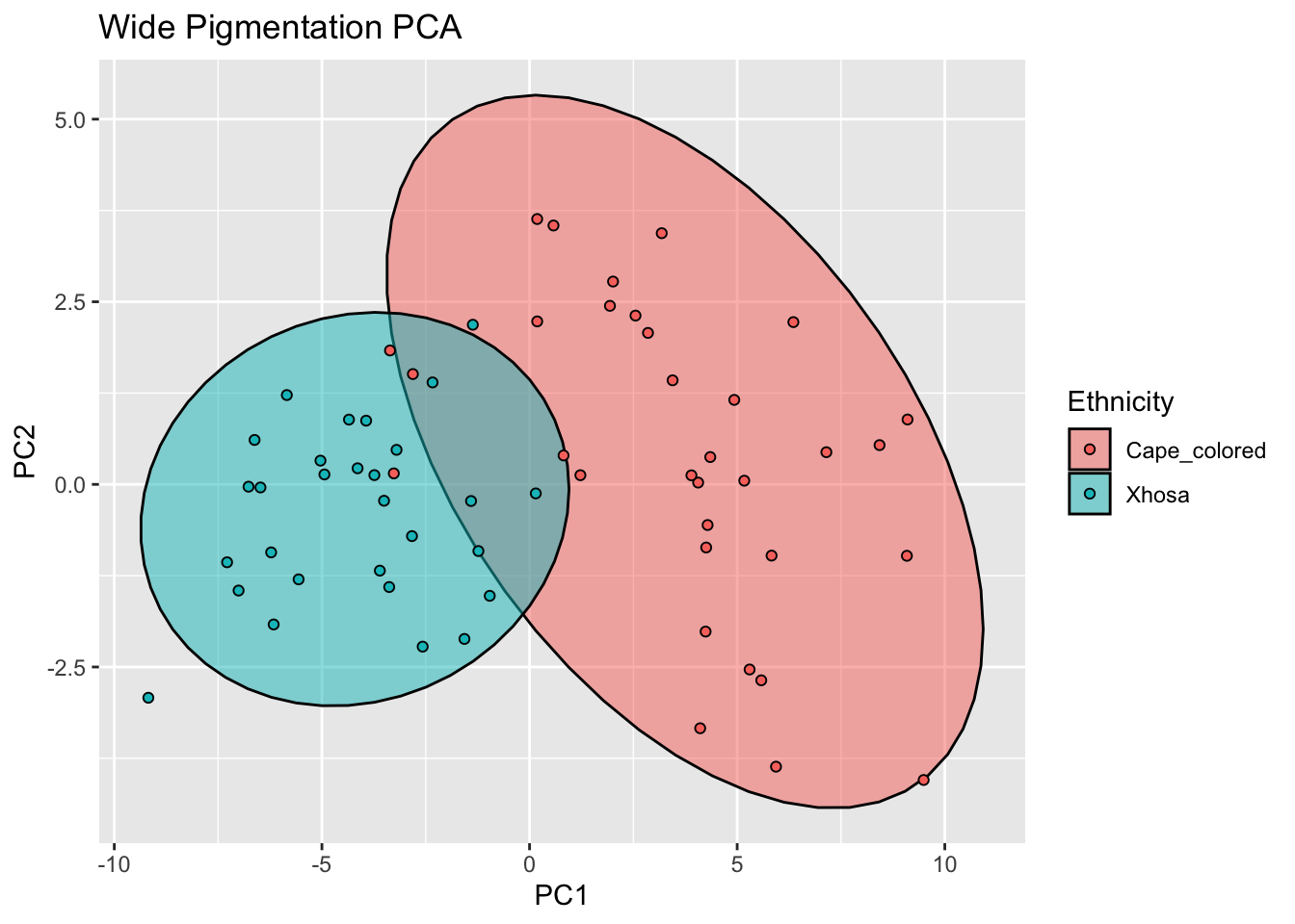
| Version | Author | Date |
|---|---|---|
| e86fbb5 | Lily Heald | 2025-04-04 |
fviz_contrib(reflectancepcaws, choice = "var", axes = 1, top = 20)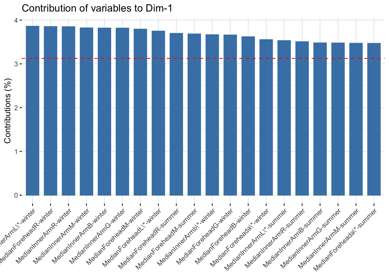
| Version | Author | Date |
|---|---|---|
| e86fbb5 | Lily Heald | 2025-04-04 |
fviz_contrib(reflectancepcaws, choice = "var", axes = 2, top = 20)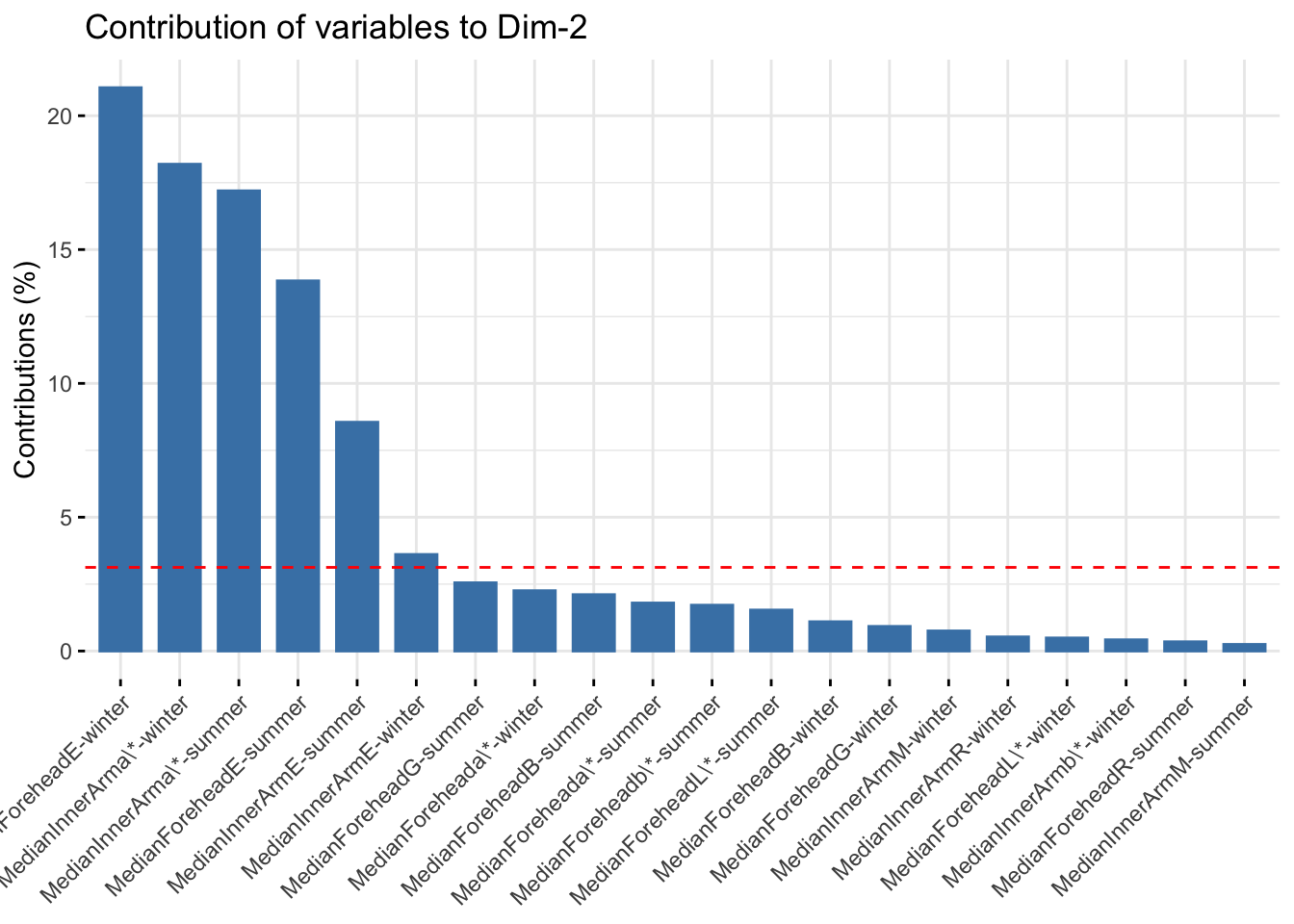
| Version | Author | Date |
|---|---|---|
| e86fbb5 | Lily Heald | 2025-04-04 |
pigmentation subset
summer_refl_metrics <- summer_data %>%
  select(matches("InnerArm|MedianForehead"))
summer_refl_metrics <- na.omit(summer_refl_metrics)

winter_refl_metrics <- winter_data %>%
  select(matches("InnerArm|MedianForehead"))
winter_refl_metrics <- na.omit(winter_refl_metrics)

six_refl_metrics <- six_week_data %>%
  select(matches("InnerArm|MedianForehead"))
six_refl_metrics <- na.omit(six_refl_metrics)
six_refl <- scale(six_refl_metrics)
six_refl_pca <- prcomp(six_refl)
summary(six_refl_pca)Importance of components:
PC1 PC2 PC3 PC4 PC5 PC6 PC7
Standard deviation 3.2964 1.5335 1.08843 0.95116 0.51710 0.41484 0.35240
Proportion of Variance 0.6792 0.1470 0.07404 0.05654 0.01671 0.01076 0.00776
Cumulative Proportion 0.6792 0.8261 0.90017 0.95672 0.97343 0.98419 0.99195
PC8 PC9 PC10 PC11 PC12 PC13 PC14
Standard deviation 0.22910 0.18667 0.12819 0.09787 0.08233 0.06270 0.04608
Proportion of Variance 0.00328 0.00218 0.00103 0.00060 0.00042 0.00025 0.00013
Cumulative Proportion 0.99523 0.99741 0.99843 0.99903 0.99945 0.99970 0.99983
PC15 PC16
Standard deviation 0.04018 0.03245
Proportion of Variance 0.00010 0.00007
Cumulative Proportion 0.99993 1.00000six_refl_pca$loadings[, 1:2]NULLfviz_eig(six_refl_pca, addlabels = TRUE)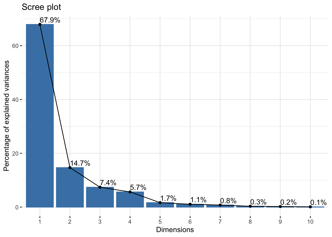
| Version | Author | Date |
|---|---|---|
| e86fbb5 | Lily Heald | 2025-04-04 |
fviz_pca_var(six_refl_pca, col.var = "black")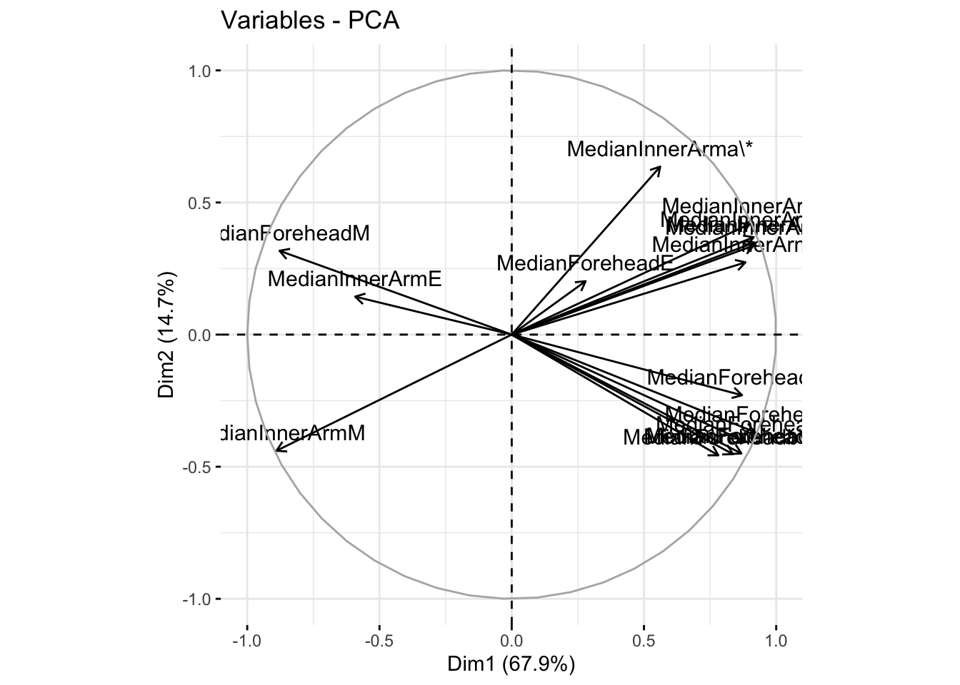
| Version | Author | Date |
|---|---|---|
| e86fbb5 | Lily Heald | 2025-04-04 |
fviz_cos2(six_refl_pca, choice = "var", axes = 1:2)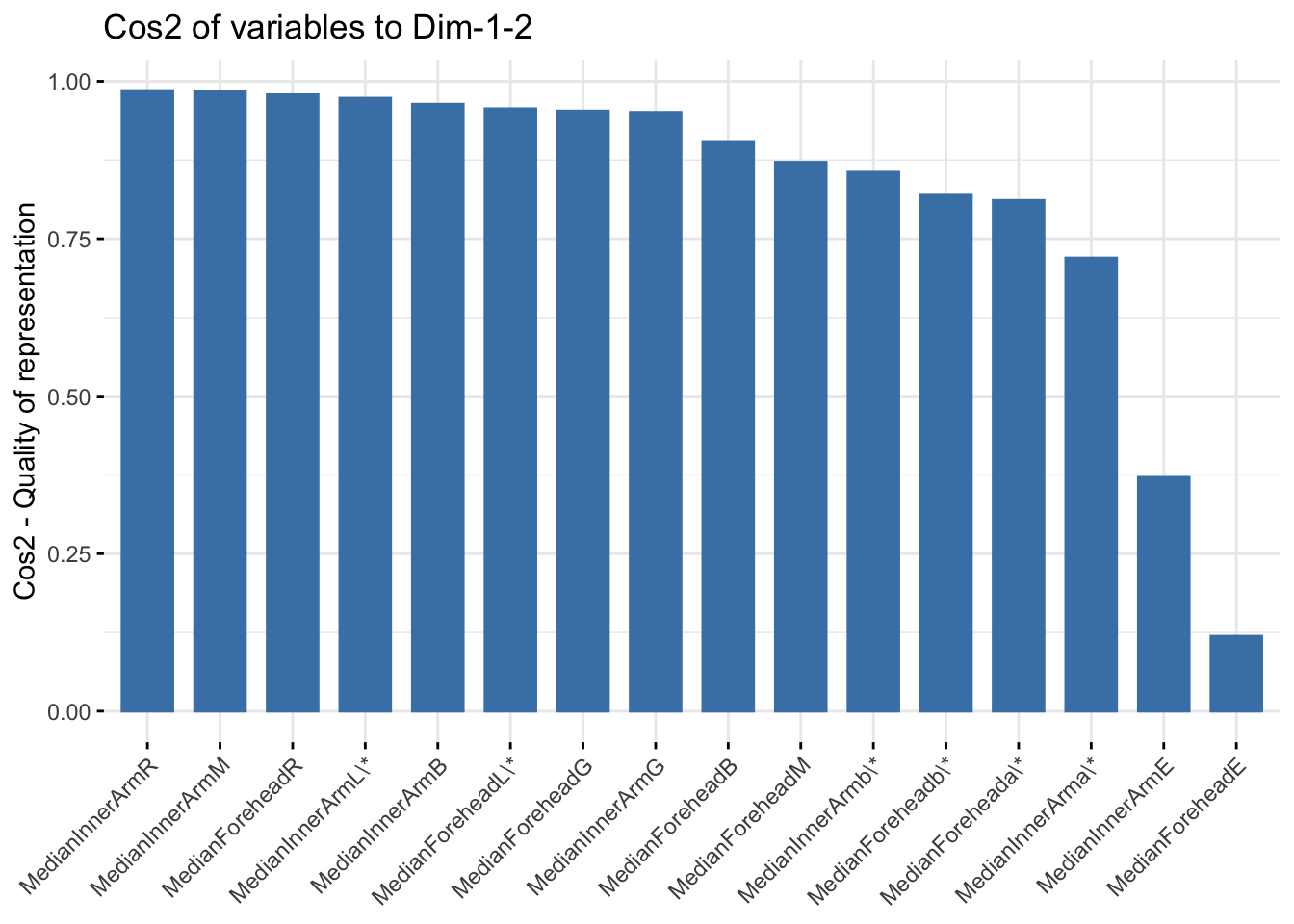
| Version | Author | Date |
|---|---|---|
| e86fbb5 | Lily Heald | 2025-04-04 |
six_pigm_comps <- as.data.frame(six_refl_pca$x)
six_pigment <- cbind(six_week_data,six_pigm_comps[,c(1,2)])

ggplot(six_pigment, aes(x=PC1, y=PC2, col = Ethnicity, fill = Ethnicity)) +
  stat_ellipse(geom = "polygon", col= "black", alpha =0.5)+
  geom_point(shape=21, col="black") +
  labs(title = "Six Week Pigmentation PCA")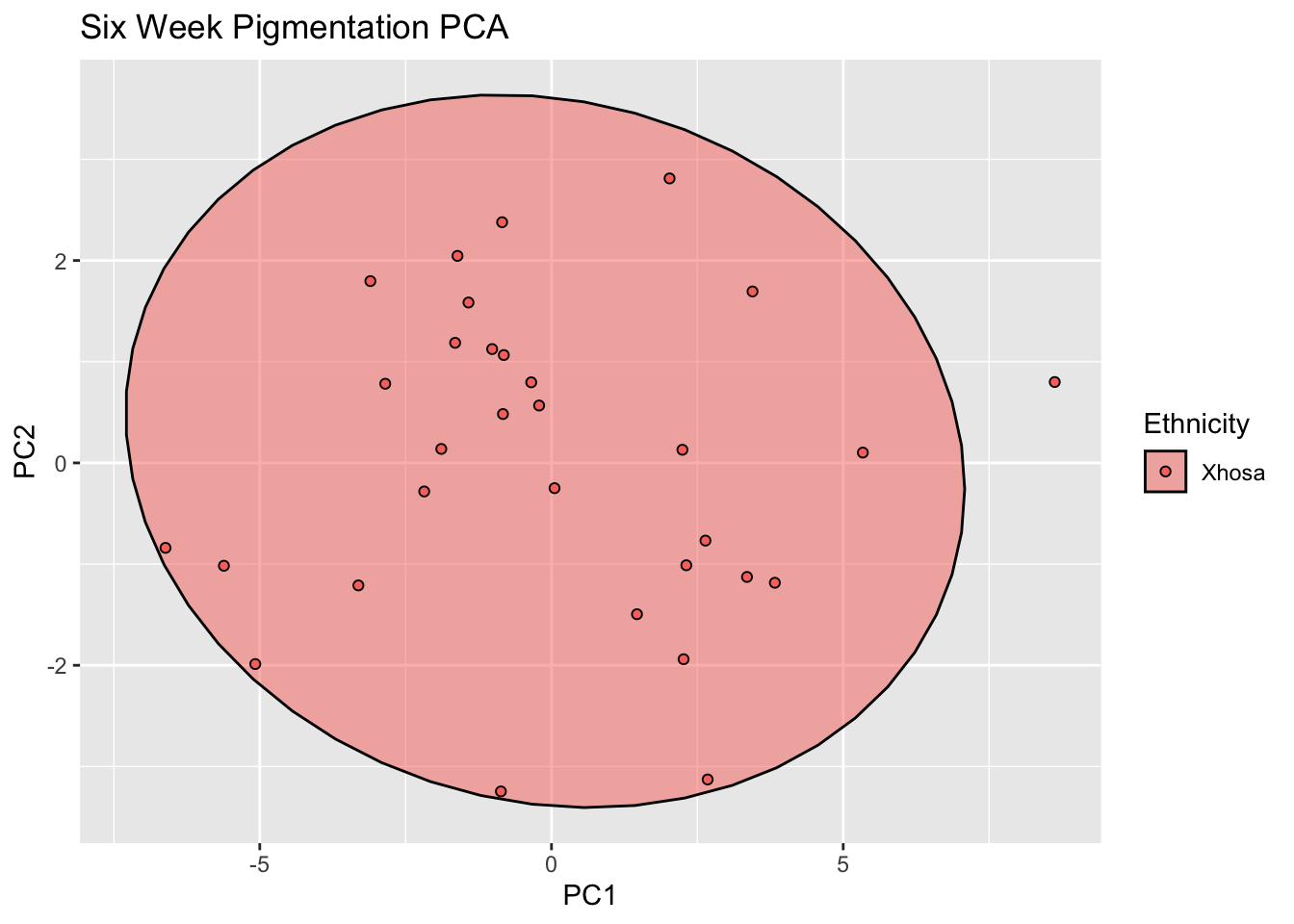
| Version | Author | Date |
|---|---|---|
| e86fbb5 | Lily Heald | 2025-04-04 |
fviz_contrib(six_refl_pca, choice = "var", axes = 1, top = 10)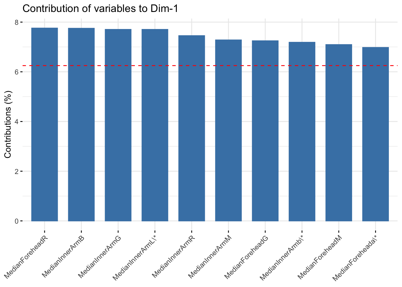
| Version | Author | Date |
|---|---|---|
| e86fbb5 | Lily Heald | 2025-04-04 |
fviz_contrib(six_refl_pca, choice = "var", axes = 2, top = 10)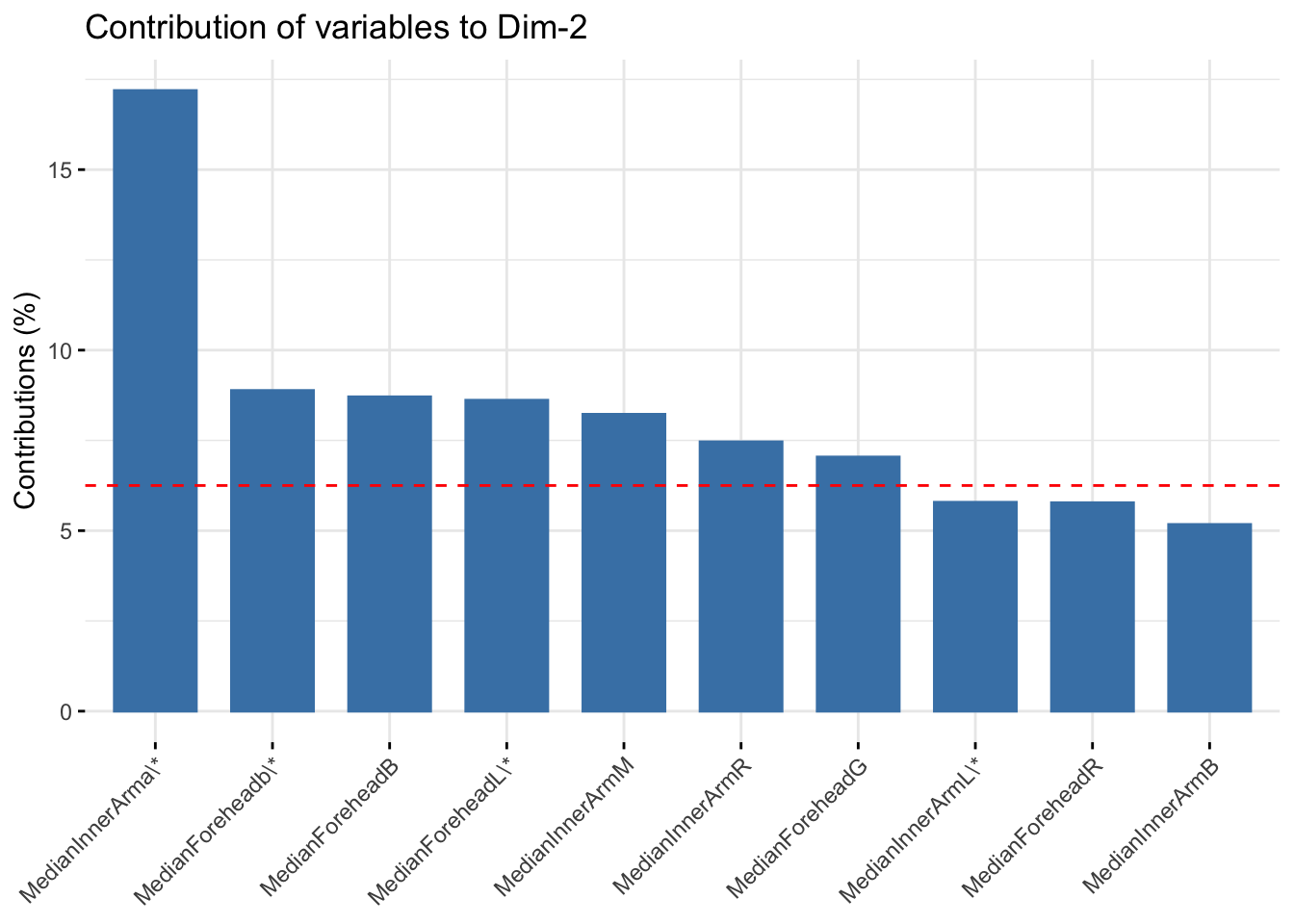
| Version | Author | Date |
|---|---|---|
| e86fbb5 | Lily Heald | 2025-04-04 |
summer_refl <- scale(summer_refl_metrics)
summer_refl_pca <- prcomp(summer_refl)
summary(summer_refl_pca)
Importance of components:
PC1 PC2 PC3 PC4 PC5 PC6 PC7
Standard deviation 3.4440 1.2656 1.16829 0.77092 0.57471 0.34227 0.21398
Proportion of Variance 0.7413 0.1001 0.08531 0.03714 0.02064 0.00732 0.00286
Cumulative Proportion 0.7413 0.8414 0.92673 0.96387 0.98451 0.99184 0.99470
PC8 PC9 PC10 PC11 PC12 PC13 PC14
Standard deviation 0.17570 0.13639 0.10998 0.09641 0.08085 0.06305 0.04166
Proportion of Variance 0.00193 0.00116 0.00076 0.00058 0.00041 0.00025 0.00011
Cumulative Proportion 0.99663 0.99779 0.99855 0.99913 0.99954 0.99978 0.99989
PC15 PC16
Standard deviation 0.03153 0.02710
Proportion of Variance 0.00006 0.00005
Cumulative Proportion 0.99995 1.00000summer_refl_pca$loadings[, 1:2]NULLfviz_eig(summer_refl_pca, addlabels = TRUE)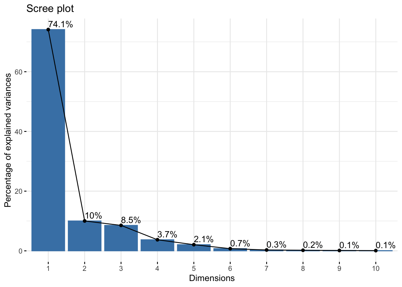
| Version | Author | Date |
|---|---|---|
| e86fbb5 | Lily Heald | 2025-04-04 |
fviz_pca_var(summer_refl_pca, col.var = "black")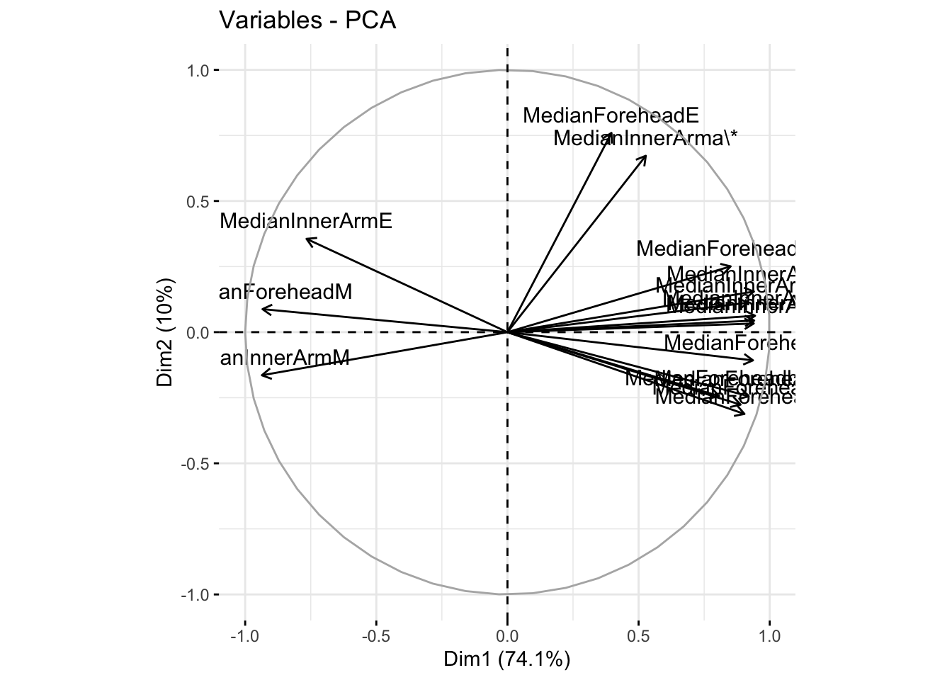
| Version | Author | Date |
|---|---|---|
| e86fbb5 | Lily Heald | 2025-04-04 |
fviz_cos2(summer_refl_pca, choice = "var", axes = 1:2)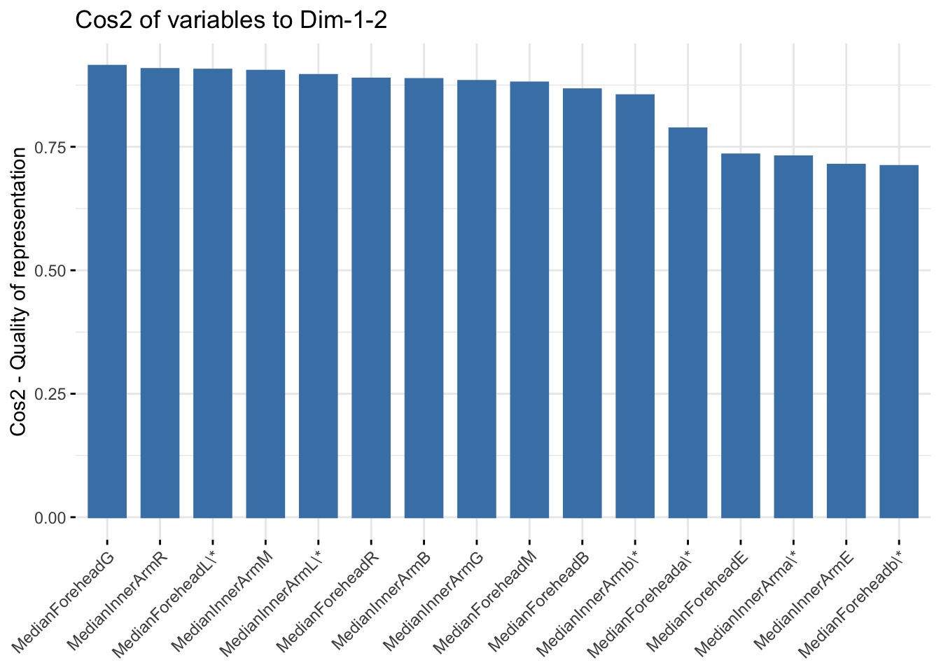
| Version | Author | Date |
|---|---|---|
| e86fbb5 | Lily Heald | 2025-04-04 |
summer_pigm_comps <- as.data.frame(summer_refl_pca$x)
summer_pigment <- cbind(summer_data,summer_pigm_comps[,c(1,2)])

ggplot(summer_pigment, aes(x=PC1, y=PC2, col = Ethnicity, fill = Ethnicity)) +
  stat_ellipse(geom = "polygon", col= "black", alpha =0.5)+
  geom_point(shape=21, col="black") +
  labs(title = "Summer Pigmentation PCA")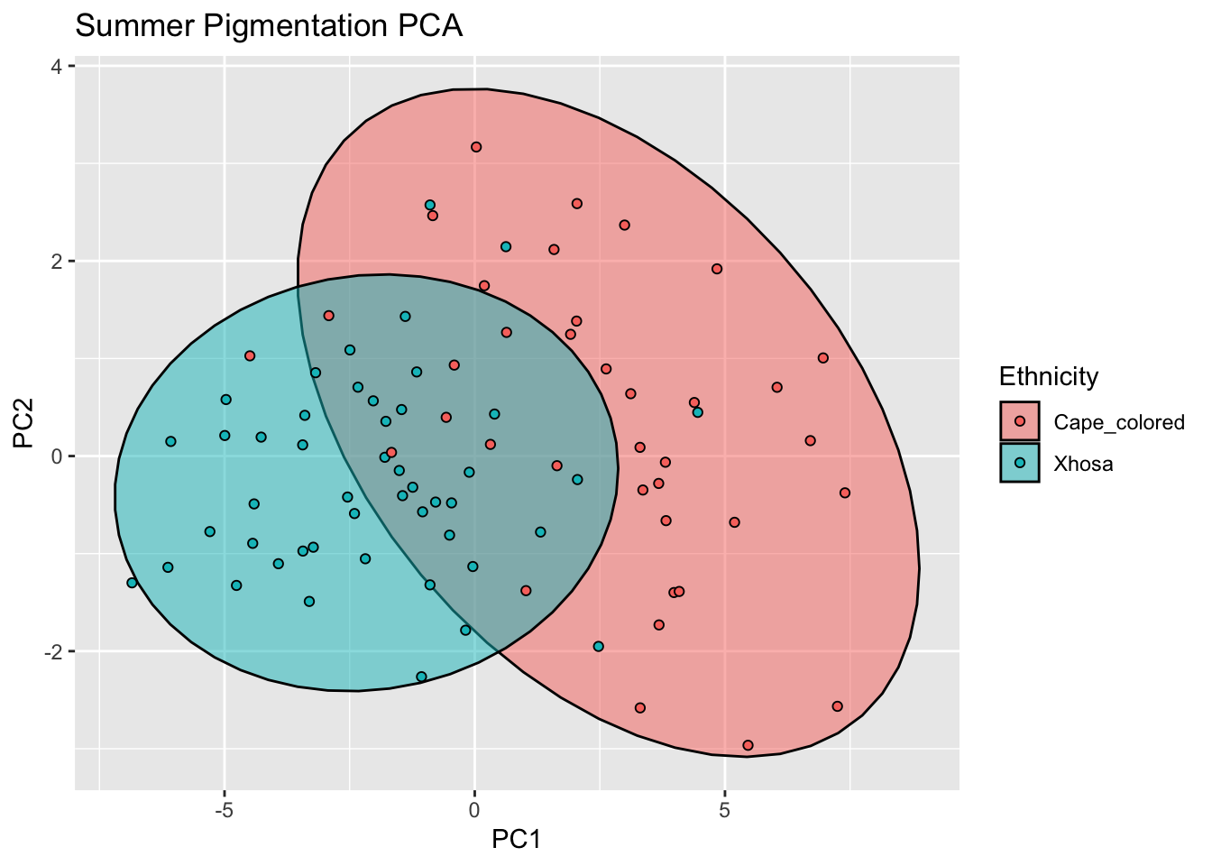
| Version | Author | Date |
|---|---|---|
| e86fbb5 | Lily Heald | 2025-04-04 |
fviz_contrib(summer_refl_pca, choice = "var", axes = 1, top = 10)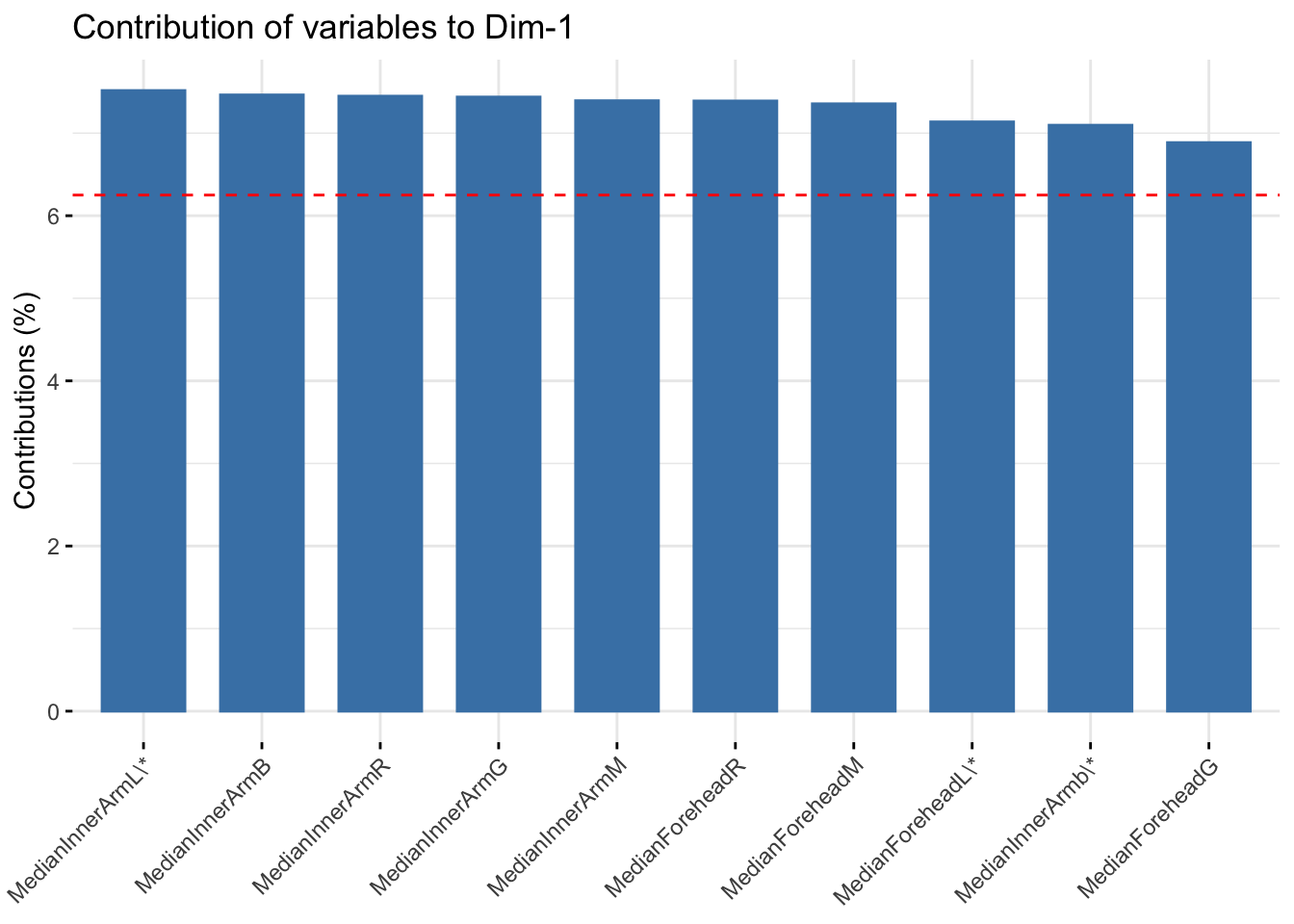
| Version | Author | Date |
|---|---|---|
| e86fbb5 | Lily Heald | 2025-04-04 |
fviz_contrib(summer_refl_pca, choice = "var", axes = 2, top = 10)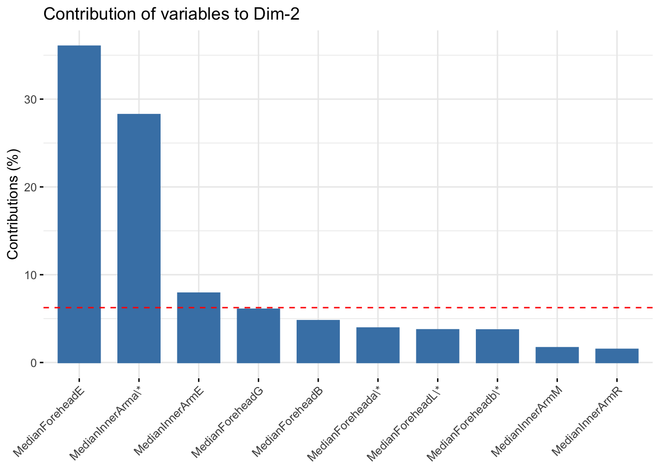
| Version | Author | Date |
|---|---|---|
| e86fbb5 | Lily Heald | 2025-04-04 |
winter_refl <- scale(winter_refl_metrics)
winter_refl_pca <- prcomp(winter_refl)
summary(winter_refl_pca)
Importance of components:
PC1 PC2 PC3 PC4 PC5 PC6 PC7
Standard deviation 3.5551 1.3839 0.80737 0.64068 0.48775 0.26632 0.15397
Proportion of Variance 0.7899 0.1197 0.04074 0.02565 0.01487 0.00443 0.00148
Cumulative Proportion 0.7899 0.9096 0.95038 0.97603 0.99090 0.99534 0.99682
PC8 PC9 PC10 PC11 PC12 PC13 PC14
Standard deviation 0.14316 0.12764 0.07986 0.06160 0.03646 0.03546 0.02830
Proportion of Variance 0.00128 0.00102 0.00040 0.00024 0.00008 0.00008 0.00005
Cumulative Proportion 0.99810 0.99912 0.99952 0.99975 0.99984 0.99991 0.99996
PC15 PC16
Standard deviation 0.01758 0.01615
Proportion of Variance 0.00002 0.00002
Cumulative Proportion 0.99998 1.00000winter_refl_pca$loadings[, 1:2]NULLfviz_eig(winter_refl_pca, addlabels = TRUE)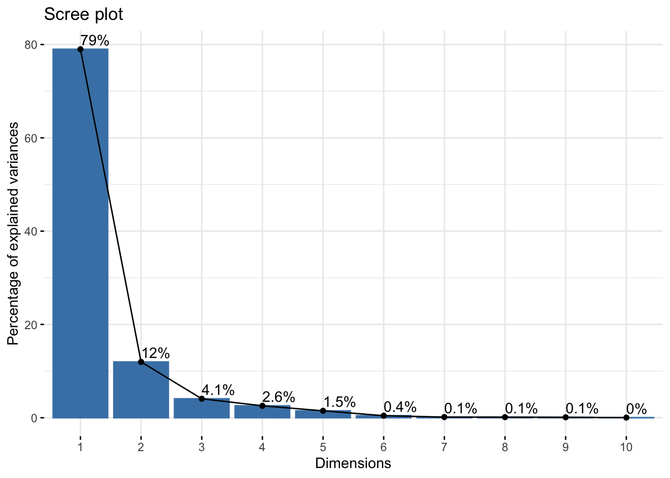
| Version | Author | Date |
|---|---|---|
| e86fbb5 | Lily Heald | 2025-04-04 |
fviz_pca_var(winter_refl_pca, col.var = "black")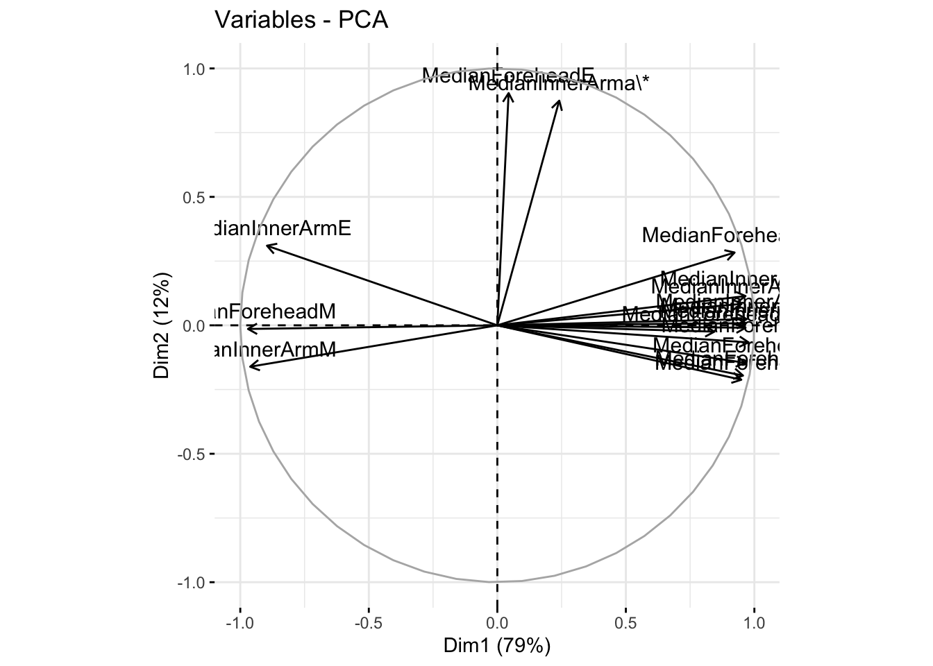
| Version | Author | Date |
|---|---|---|
| e86fbb5 | Lily Heald | 2025-04-04 |
fviz_cos2(winter_refl_pca, choice = "var", axes = 1:2)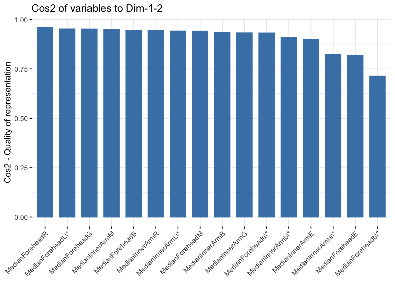
| Version | Author | Date |
|---|---|---|
| e86fbb5 | Lily Heald | 2025-04-04 |
winter_pigm_comps <- as.data.frame(winter_refl_pca$x)
winter_pigment <- cbind(winter_data,winter_pigm_comps[,c(1,2)])

ggplot(winter_pigment, aes(x=PC1, y=PC2, col = Ethnicity, fill = Ethnicity)) +
  stat_ellipse(geom = "polygon", col= "black", alpha =0.5)+
  geom_point(shape=21, col="black") +
  labs(title = "Winter Pigmentation PCA")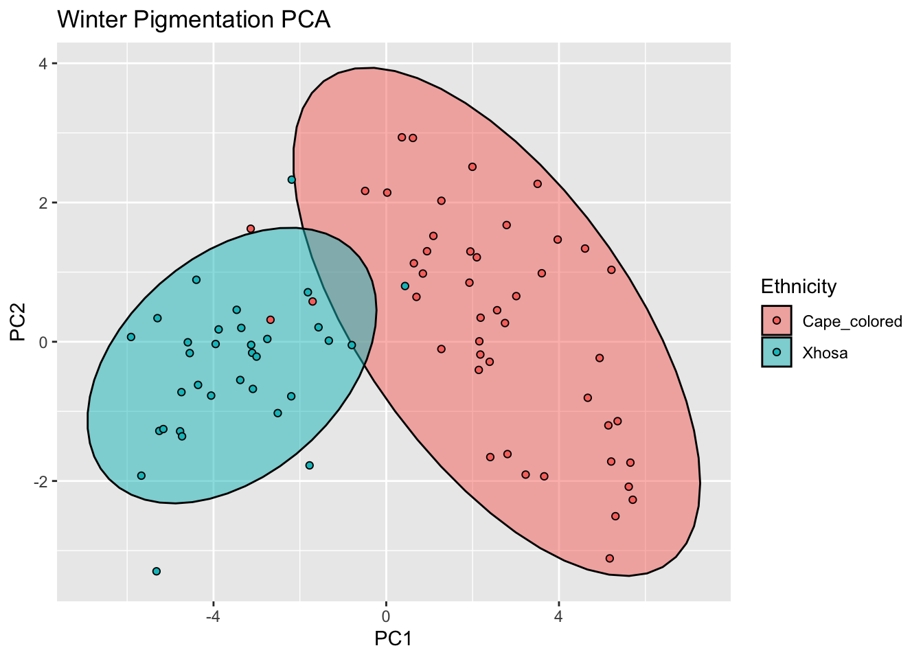
| Version | Author | Date |
|---|---|---|
| e86fbb5 | Lily Heald | 2025-04-04 |
fviz_contrib(winter_refl_pca, choice = "var", axes = 1, top = 10)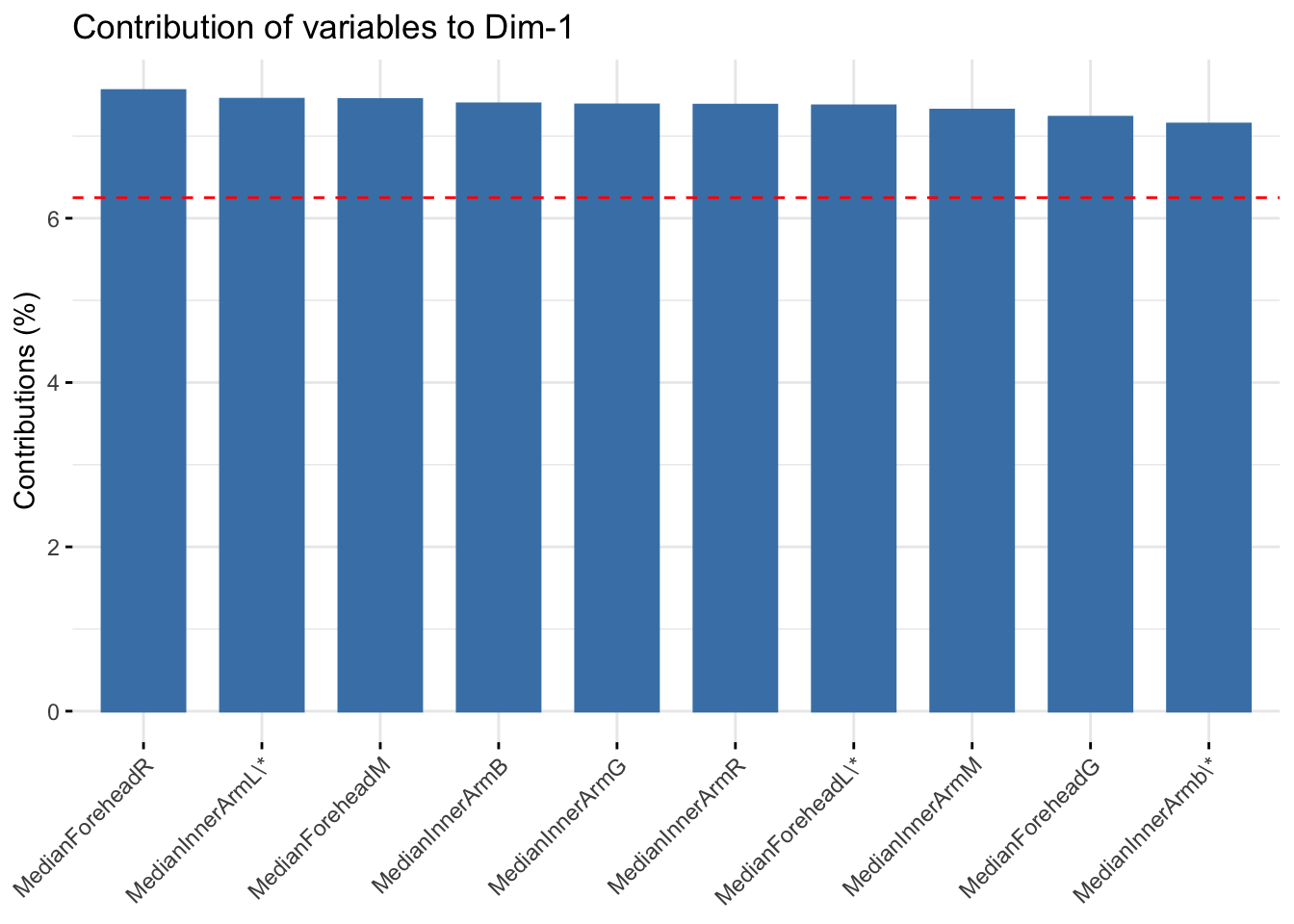
| Version | Author | Date |
|---|---|---|
| e86fbb5 | Lily Heald | 2025-04-04 |
fviz_contrib(winter_refl_pca, choice = "var", axes = 2, top = 10)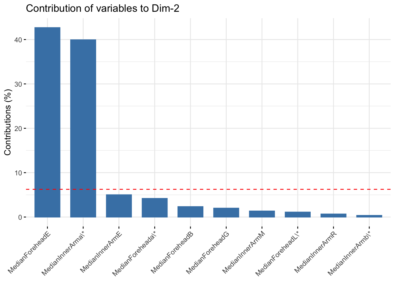
| Version | Author | Date |
|---|---|---|
| e86fbb5 | Lily Heald | 2025-04-04 |
RGB subset
summer_winter_clean <- na.omit(summer_winter)
reflectance_rgb_ws <- summer_winter_clean %>%
  select(matches("MedianForeheadR|MedianForeheadG|MedianForeheadB|InnerArmR|InnerArmG|InnerArmB", ignore.case = FALSE))

reflectance4 <- scale(reflectance_rgb_ws)
reflectancergbws <- prcomp(reflectance4)
summary(reflectancergbws)
Importance of components:
PC1 PC2 PC3 PC4 PC5 PC6 PC7
Standard deviation 3.2234 0.9250 0.64032 0.4749 0.23334 0.17127 0.11920
Proportion of Variance 0.8658 0.0713 0.03417 0.0188 0.00454 0.00244 0.00118
Cumulative Proportion 0.8658 0.9371 0.97131 0.9901 0.99464 0.99709 0.99827
PC8 PC9 PC10 PC11 PC12
Standard deviation 0.08932 0.07877 0.06799 0.03813 0.02223
Proportion of Variance 0.00066 0.00052 0.00039 0.00012 0.00004
Cumulative Proportion 0.99894 0.99945 0.99984 0.99996 1.00000reflectancergbws$loadings[, 1:2]NULLfviz_eig(reflectancergbws, addlabels = TRUE)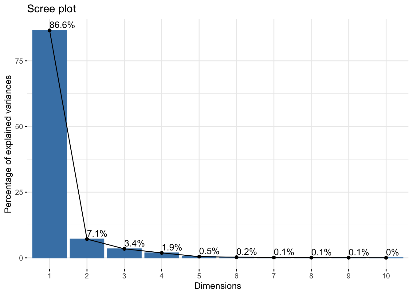
| Version | Author | Date |
|---|---|---|
| e86fbb5 | Lily Heald | 2025-04-04 |
fviz_pca_var(reflectancergbws, col.var = "black")
| Version | Author | Date |
|---|---|---|
| e86fbb5 | Lily Heald | 2025-04-04 |
fviz_cos2(reflectancergbws, choice = "var", axes = 1:2)
| Version | Author | Date |
|---|---|---|
| e86fbb5 | Lily Heald | 2025-04-04 |
wsrgbcomps <- as.data.frame(reflectancergbws$x)
rgb_ws_bind <- cbind(summer_winter_clean,wsrgbcomps[,c(1,2)])
rgb_ws_bind <- rgb_ws_bind %>%
  select(-matches("SkinReflectance"))
rgb_ws_bind <- rgb_ws_bind %>%
  select(-"Ethnicity-winter")
names(rgb_ws_bind)[names(rgb_ws_bind) == 'Ethnicity-summer'] <- 'Ethnicity'


ggplot(rgb_ws_bind, aes(x=PC1, y=PC2, col = Ethnicity, fill = Ethnicity)) +
  stat_ellipse(geom = "polygon", col= "black", alpha =0.5)+
  geom_point(shape=21, col="black") +
  labs(title = "Wide Pigmentation PCA")
| Version | Author | Date |
|---|---|---|
| e86fbb5 | Lily Heald | 2025-04-04 |
fviz_contrib(reflectancergbws, choice = "var", axes = 1, top = 20)
| Version | Author | Date |
|---|---|---|
| e86fbb5 | Lily Heald | 2025-04-04 |
fviz_contrib(reflectancergbws, choice = "var", axes = 2, top = 20)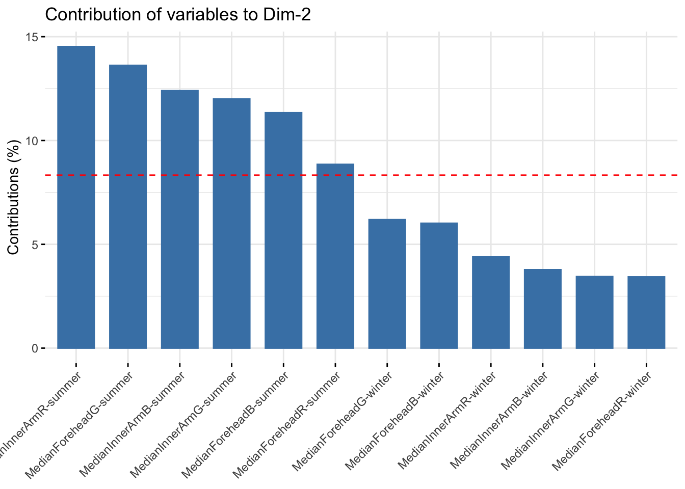
| Version | Author | Date |
|---|---|---|
| e86fbb5 | Lily Heald | 2025-04-04 |
summer_rgb <- summer_data %>%
  select(matches("ForeheadR|ForeheadG|ForeheadB|InnerArmR|InnerArmG|InnerArmB", ignore.case = FALSE))
summer_rgb <- na.omit(summer_rgb)

winter_rgb <- winter_data %>%
  select(matches("ForeheadR|ForeheadG|ForeheadB|InnerArmR|InnerArmG|InnerArmB", ignore.case = FALSE))
winter_rgb <- na.omit(winter_rgb)

six_rgb <- six_week_data %>%
  select(matches("ForeheadR|ForeheadG|ForeheadB|InnerArmR|InnerArmG|InnerArmB", ignore.case = FALSE))
six_rgb <- na.omit(six_rgb)
winter_rgb_scale <- scale(winter_rgb)
winter_rgb_pca <- prcomp(winter_rgb_scale)
summary(winter_rgb_pca)Importance of components:
PC1 PC2 PC3 PC4 PC5 PC6
Standard deviation 2.3720 0.58112 0.15130 0.08075 0.07684 0.01941
Proportion of Variance 0.9378 0.05628 0.00382 0.00109 0.00098 0.00006
Cumulative Proportion 0.9378 0.99405 0.99787 0.99895 0.99994 1.00000winter_rgb_pca$loadings[, 1:2]NULLfviz_eig(winter_rgb_pca, addlabels = TRUE)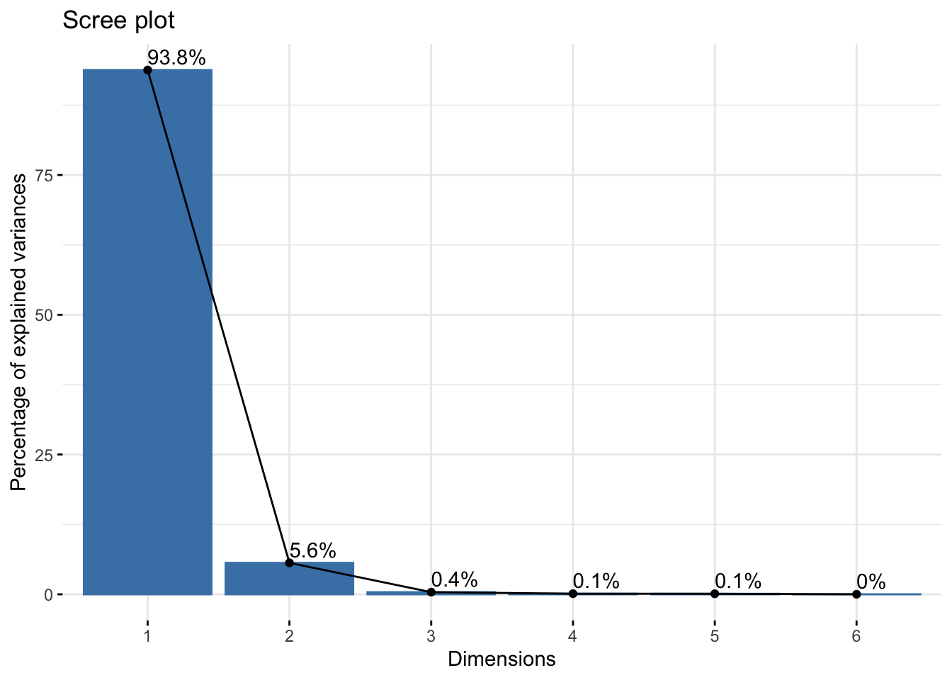
| Version | Author | Date |
|---|---|---|
| e86fbb5 | Lily Heald | 2025-04-04 |
fviz_pca_var(winter_rgb_pca, col.var = "black")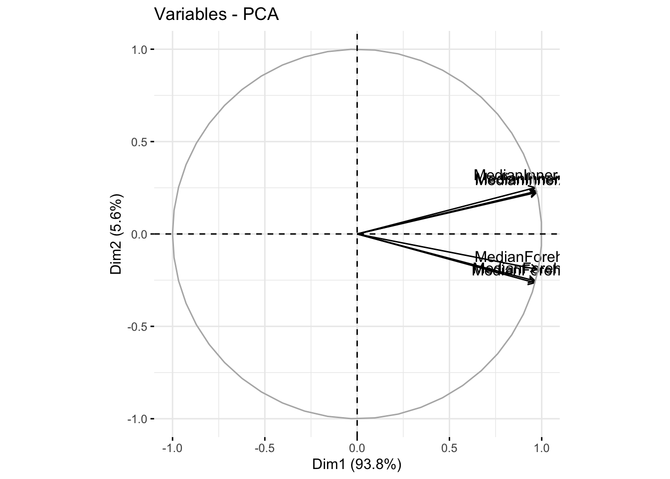
| Version | Author | Date |
|---|---|---|
| e86fbb5 | Lily Heald | 2025-04-04 |
fviz_cos2(winter_rgb_pca, choice = "var", axes = 1:2)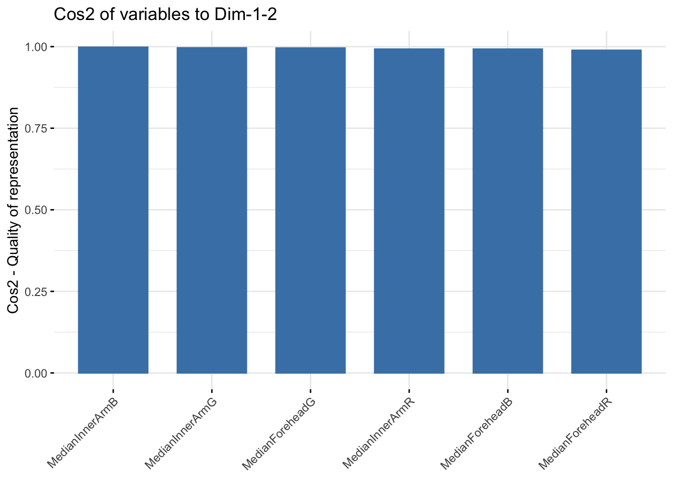
| Version | Author | Date |
|---|---|---|
| e86fbb5 | Lily Heald | 2025-04-04 |
winter_rgb_comps <- as.data.frame(winter_rgb_pca$x)
winter_rgb_new <- cbind(winter_data,winter_rgb_comps[,c(1,2)])

ggplot(winter_rgb_new, aes(x=PC1, y=PC2, col = Ethnicity, fill = Ethnicity)) +
  stat_ellipse(geom = "polygon", col= "black", alpha =0.5)+
  geom_point(shape=21, col="black") +
  labs(title = "Winter RGB PCA")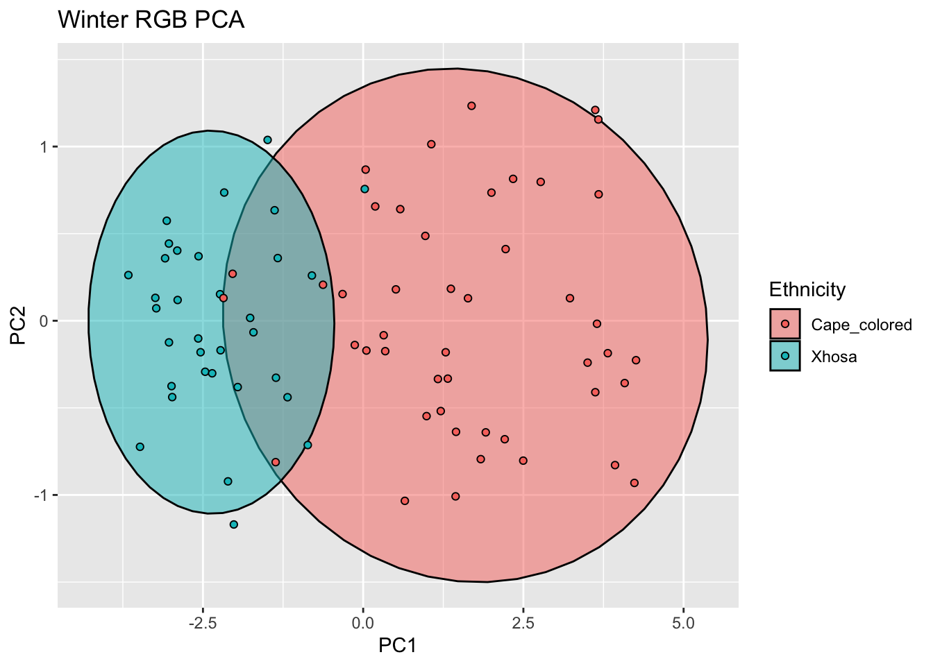
| Version | Author | Date |
|---|---|---|
| e86fbb5 | Lily Heald | 2025-04-04 |
fviz_contrib(winter_rgb_pca, choice = "var", axes = 1, top = 10)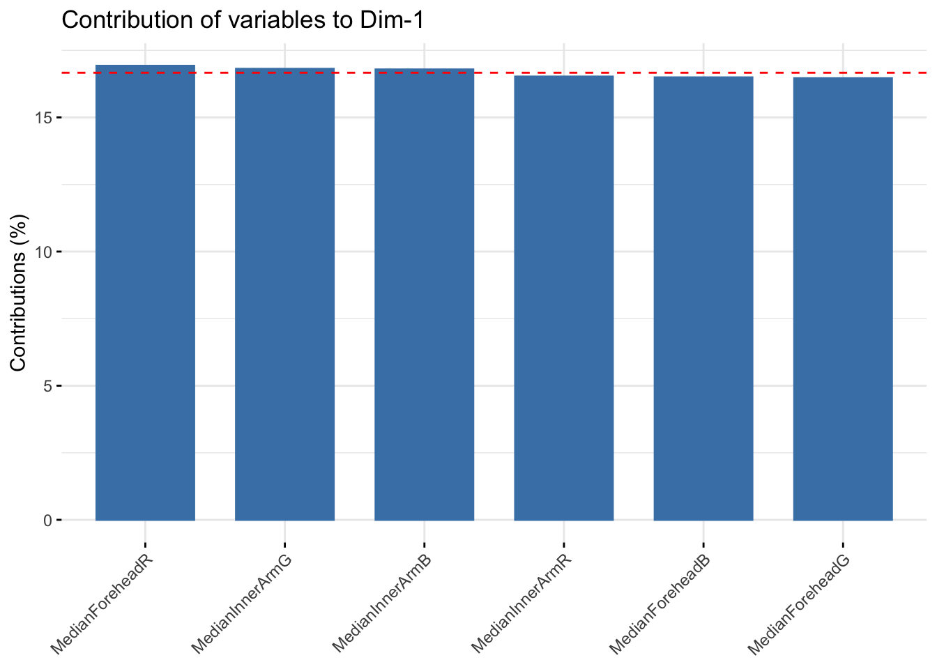
| Version | Author | Date |
|---|---|---|
| e86fbb5 | Lily Heald | 2025-04-04 |
fviz_contrib(winter_rgb_pca, choice = "var", axes = 2, top = 10)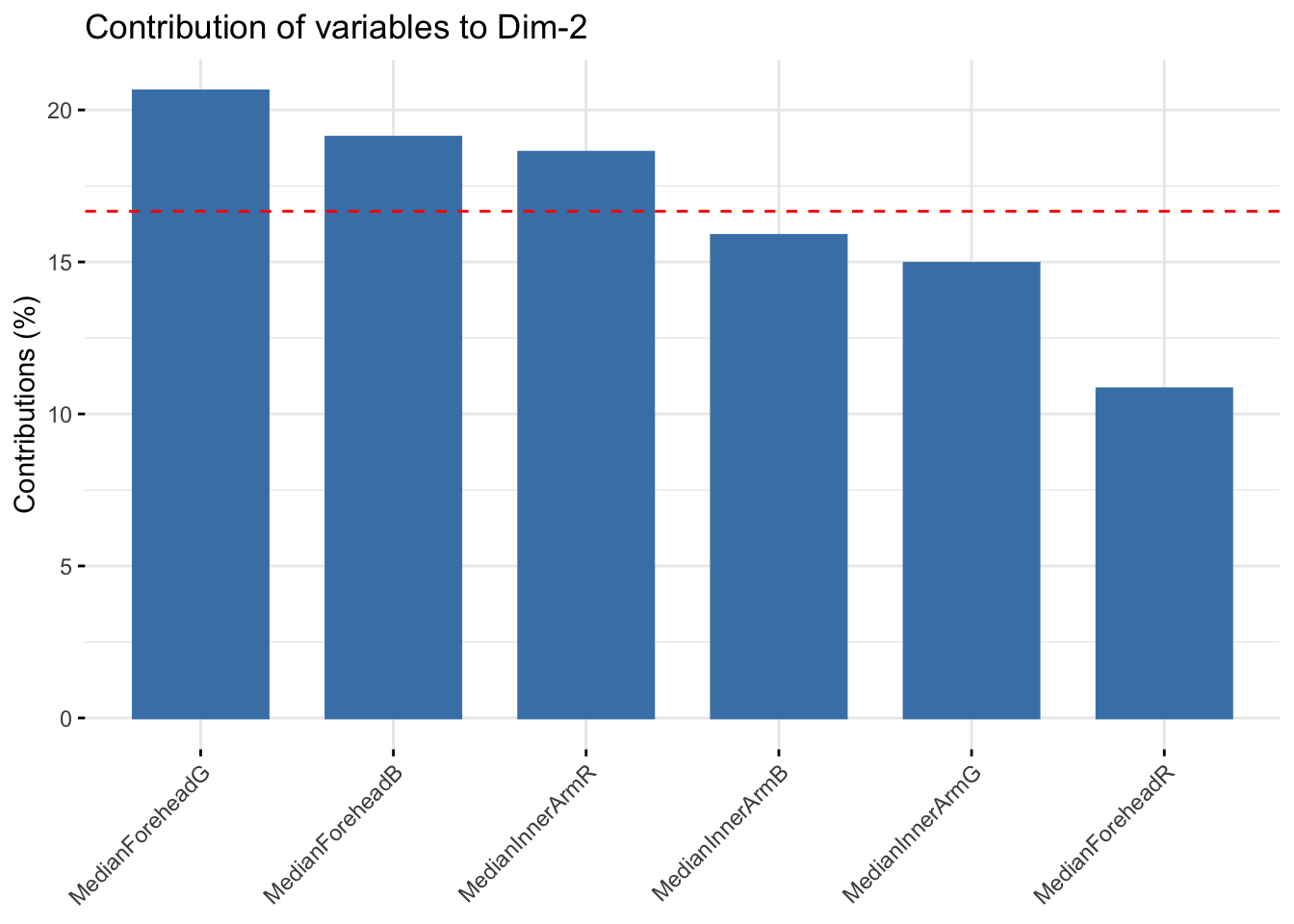
| Version | Author | Date |
|---|---|---|
| e86fbb5 | Lily Heald | 2025-04-04 |
summer_rgb_scale <- scale(summer_rgb)
summer_rgb_pca <- prcomp(summer_rgb_scale)
summary(summer_rgb_pca)
Importance of components:
PC1 PC2 PC3 PC4 PC5 PC6
Standard deviation 2.286 0.8242 0.23805 0.15859 0.1067 0.04116
Proportion of Variance 0.871 0.1132 0.00944 0.00419 0.0019 0.00028
Cumulative Proportion 0.871 0.9842 0.99363 0.99782 0.9997 1.00000summer_rgb_pca$loadings[, 1:2]NULLfviz_eig(summer_rgb_pca, addlabels = TRUE)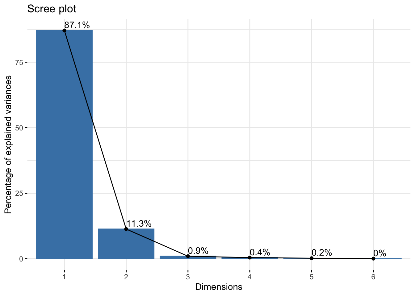
| Version | Author | Date |
|---|---|---|
| e86fbb5 | Lily Heald | 2025-04-04 |
fviz_pca_var(summer_rgb_pca, col.var = "black")
| Version | Author | Date |
|---|---|---|
| e86fbb5 | Lily Heald | 2025-04-04 |
fviz_cos2(summer_rgb_pca, choice = "var", axes = 1:2)
| Version | Author | Date |
|---|---|---|
| e86fbb5 | Lily Heald | 2025-04-04 |
summer_rgb_comps <- as.data.frame(summer_rgb_pca$x)
summer_rgb_new <- cbind(summer_data,summer_rgb_comps[,c(1,2)])

ggplot(summer_rgb_new, aes(x=PC1, y=PC2, col = Ethnicity, fill = Ethnicity)) +
  stat_ellipse(geom = "polygon", col= "black", alpha =0.5)+
  geom_point(shape=21, col="black") +
  labs(title = "Summer RGB PCA")
| Version | Author | Date |
|---|---|---|
| e86fbb5 | Lily Heald | 2025-04-04 |
fviz_contrib(summer_rgb_pca, choice = "var", axes = 1, top = 10)
| Version | Author | Date |
|---|---|---|
| e86fbb5 | Lily Heald | 2025-04-04 |
fviz_contrib(summer_rgb_pca, choice = "var", axes = 2, top = 10)
| Version | Author | Date |
|---|---|---|
| e86fbb5 | Lily Heald | 2025-04-04 |
six_rgb_scale <- scale(six_rgb)
six_rgb_pca <- prcomp(six_rgb_scale)
summary(six_rgb_pca)
Importance of components:
PC1 PC2 PC3 PC4 PC5 PC6
Standard deviation 2.2119 1.0170 0.17400 0.14471 0.13214 0.06648
Proportion of Variance 0.8154 0.1724 0.00505 0.00349 0.00291 0.00074
Cumulative Proportion 0.8154 0.9878 0.99286 0.99635 0.99926 1.00000six_rgb_pca$loadings[, 1:2]NULLfviz_eig(six_rgb_pca, addlabels = TRUE)
| Version | Author | Date |
|---|---|---|
| e86fbb5 | Lily Heald | 2025-04-04 |
fviz_pca_var(six_rgb_pca, col.var = "black")
| Version | Author | Date |
|---|---|---|
| e86fbb5 | Lily Heald | 2025-04-04 |
fviz_cos2(six_rgb_pca, choice = "var", axes = 1:2)
| Version | Author | Date |
|---|---|---|
| e86fbb5 | Lily Heald | 2025-04-04 |
six_rgb_comps <- as.data.frame(six_rgb_pca$x)
six_rgb_new <- cbind(six_week_data,six_rgb_comps[,c(1,2)])

ggplot(six_rgb_new, aes(x=PC1, y=PC2, col = Ethnicity, fill = Ethnicity)) +
  stat_ellipse(geom = "polygon", col= "black", alpha =0.5)+
  geom_point(shape=21, col="black") +
  labs(title = "Six Week RGB PCA")
| Version | Author | Date |
|---|---|---|
| e86fbb5 | Lily Heald | 2025-04-04 |
fviz_contrib(six_rgb_pca, choice = "var", axes = 1, top = 10)
| Version | Author | Date |
|---|---|---|
| e86fbb5 | Lily Heald | 2025-04-04 |
fviz_contrib(six_rgb_pca, choice = "var", axes = 2, top = 10)
| Version | Author | Date |
|---|---|---|
| e86fbb5 | Lily Heald | 2025-04-04 |
CIElab subset
summer_winter_clean <- na.omit(summer_winter)
reflectance_cie_ws <- summer_winter_clean %>%
  select(matches("ForeheadL|Foreheada|Foreheadb|InnerArmL|InnerArma|InnerArmb", ignore.case = FALSE))

reflectance5 <- scale(reflectance_cie_ws)
reflectanceciews <- prcomp(reflectance5)
summary(reflectanceciews)
Importance of components:
PC1 PC2 PC3 PC4 PC5 PC6 PC7
Standard deviation 2.9442 1.2216 0.6971 0.64830 0.56414 0.45873 0.38123
Proportion of Variance 0.7223 0.1244 0.0405 0.03502 0.02652 0.01754 0.01211
Cumulative Proportion 0.7223 0.8467 0.8872 0.92222 0.94874 0.96628 0.97839
PC8 PC9 PC10 PC11 PC12
Standard deviation 0.29699 0.24598 0.2298 0.17889 0.16070
Proportion of Variance 0.00735 0.00504 0.0044 0.00267 0.00215
Cumulative Proportion 0.98574 0.99078 0.9952 0.99785 1.00000reflectanceciews$loadings[, 1:2]NULLfviz_eig(reflectanceciews, addlabels = TRUE)
| Version | Author | Date |
|---|---|---|
| e86fbb5 | Lily Heald | 2025-04-04 |
fviz_pca_var(reflectanceciews, col.var = "black")
| Version | Author | Date |
|---|---|---|
| e86fbb5 | Lily Heald | 2025-04-04 |
fviz_cos2(reflectanceciews, choice = "var", axes = 1:2)
| Version | Author | Date |
|---|---|---|
| e86fbb5 | Lily Heald | 2025-04-04 |
wsciecomps <- as.data.frame(reflectanceciews$x)
cie_ws_bind <- cbind(summer_winter_clean,wsciecomps[,c(1,2)])
cie_ws_bind <- rgb_ws_bind %>%
  select(-matches("SkinReflectance"))

ggplot(cie_ws_bind, aes(x=PC1, y=PC2, col = Ethnicity, fill = Ethnicity)) +
  stat_ellipse(geom = "polygon", col= "black", alpha =0.5)+
  geom_point(shape=21, col="black") +
  labs(title = "Wide Pigmentation PCA")
| Version | Author | Date |
|---|---|---|
| e86fbb5 | Lily Heald | 2025-04-04 |
fviz_contrib(reflectanceciews, choice = "var", axes = 1, top = 20)
| Version | Author | Date |
|---|---|---|
| e86fbb5 | Lily Heald | 2025-04-04 |
fviz_contrib(reflectanceciews, choice = "var", axes = 2, top = 20)
| Version | Author | Date |
|---|---|---|
| e86fbb5 | Lily Heald | 2025-04-04 |
summer_cie <- summer_data %>%
  select(matches("ForeheadL|Foreheada|Foreheadb|InnerArmL|InnerArma|InnerArmb", ignore.case = FALSE))
summer_cie <- na.omit(summer_cie)

winter_cie <- winter_data %>%
  select(matches("ForeheadL|Foreheada|Foreheadb|InnerArmL|InnerArma|InnerArmb", ignore.case = FALSE))
winter_cie <- na.omit(winter_cie)

six_cie <- six_week_data %>%
  select(matches("ForeheadL|Foreheada|Foreheadb|InnerArmL|InnerArma|InnerArmb", ignore.case = FALSE))
six_cie <- na.omit(six_cie)
winter_cie_scale <- scale(winter_cie)
winter_cie_pca <- prcomp(winter_cie_scale)
summary(winter_cie_pca)Importance of components:
PC1 PC2 PC3 PC4 PC5 PC6
Standard deviation 2.1257 0.9808 0.5304 0.36540 0.2486 0.20736
Proportion of Variance 0.7531 0.1603 0.0469 0.02225 0.0103 0.00717
Cumulative Proportion 0.7531 0.9134 0.9603 0.98253 0.9928 1.00000winter_cie_pca$loadings[, 1:2]NULLfviz_eig(winter_cie_pca, addlabels = TRUE)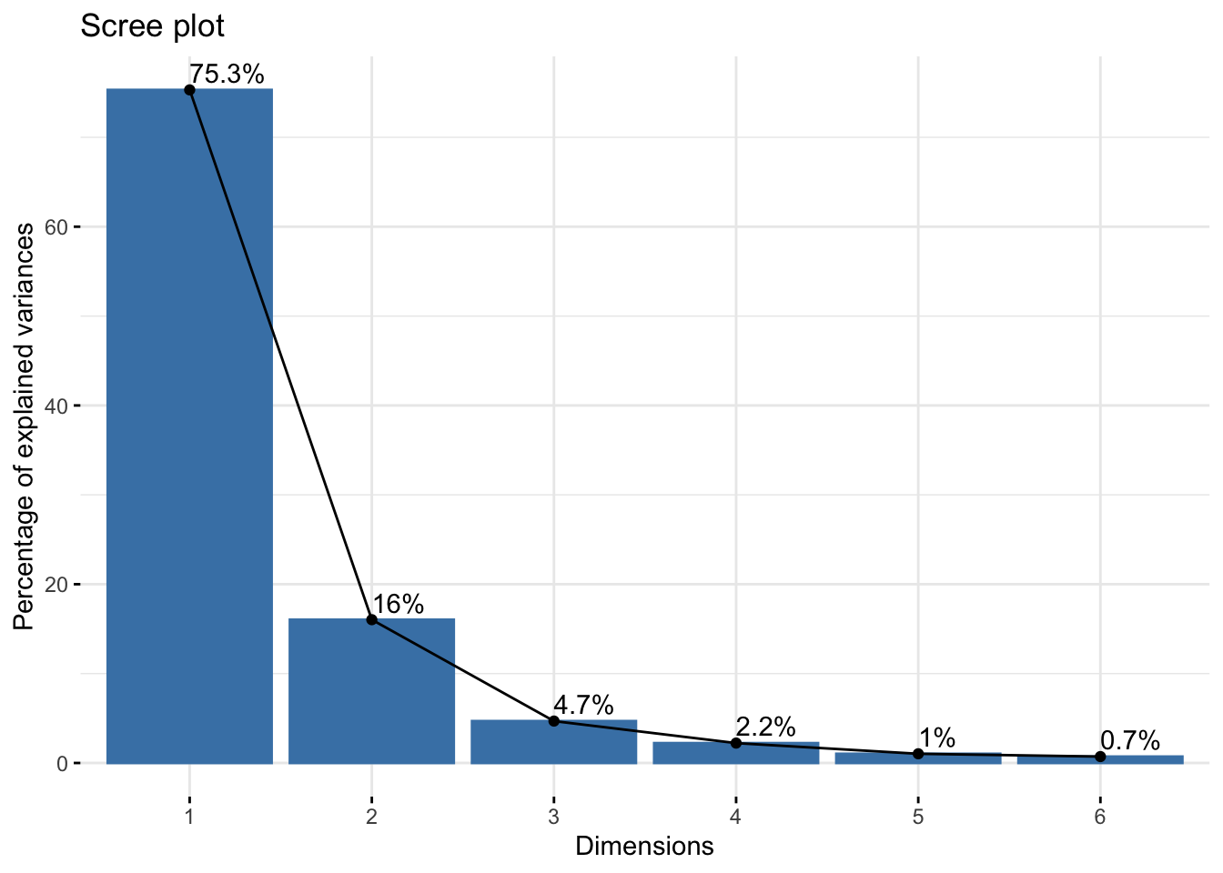
| Version | Author | Date |
|---|---|---|
| e86fbb5 | Lily Heald | 2025-04-04 |
fviz_pca_var(winter_cie_pca, col.var = "black")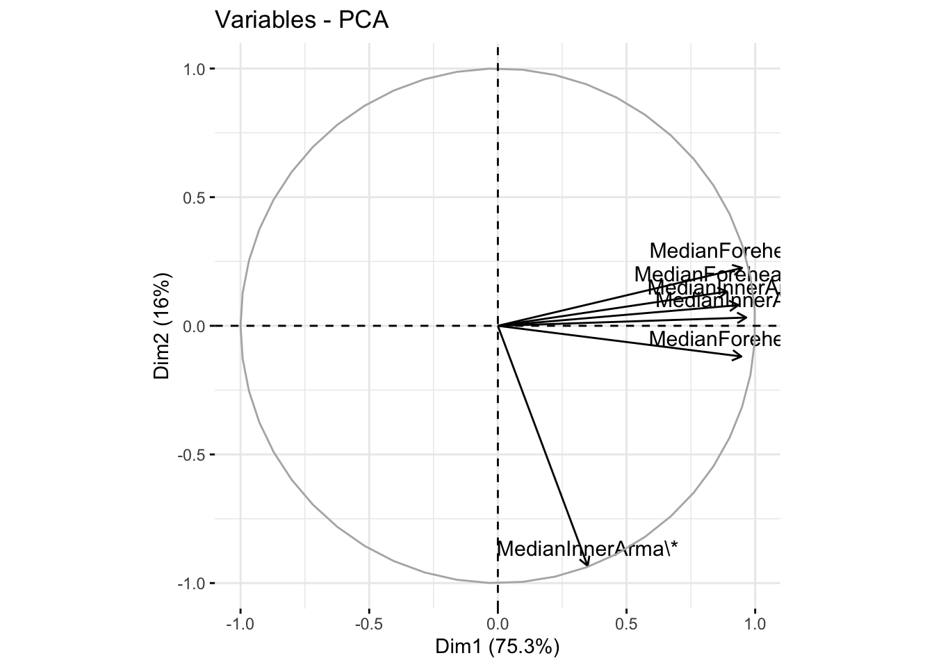
| Version | Author | Date |
|---|---|---|
| e86fbb5 | Lily Heald | 2025-04-04 |
fviz_cos2(winter_cie_pca, choice = "var", axes = 1:2)
| Version | Author | Date |
|---|---|---|
| e86fbb5 | Lily Heald | 2025-04-04 |
winter_cie_comps <- as.data.frame(winter_cie_pca$x)
winter_cie_new <- cbind(winter_data,winter_cie_comps[,c(1,2)])

ggplot(winter_cie_new, aes(x=PC1, y=PC2, col = Ethnicity, fill = Ethnicity)) +
  stat_ellipse(geom = "polygon", col= "black", alpha =0.5)+
  geom_point(shape=21, col="black") +
  labs(title = "Winter CIELAB PCA")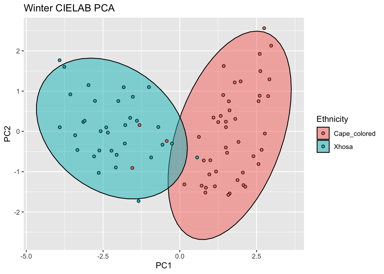
| Version | Author | Date |
|---|---|---|
| e86fbb5 | Lily Heald | 2025-04-04 |
fviz_contrib(winter_cie_pca, choice = "var", axes = 1, top = 10)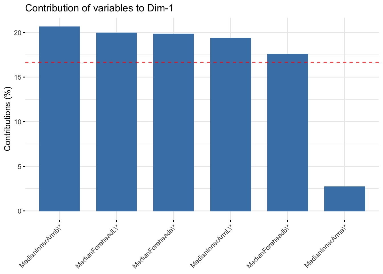
| Version | Author | Date |
|---|---|---|
| e86fbb5 | Lily Heald | 2025-04-04 |
fviz_contrib(winter_cie_pca, choice = "var", axes = 2, top = 10)
| Version | Author | Date |
|---|---|---|
| e86fbb5 | Lily Heald | 2025-04-04 |
summer_cie_scale <- scale(summer_cie)
summer_cie_pca <- prcomp(summer_cie_scale)
summary(summer_cie_pca)
Importance of components:
PC1 PC2 PC3 PC4 PC5 PC6
Standard deviation 2.0841 0.9045 0.60937 0.53086 0.35079 0.24908
Proportion of Variance 0.7239 0.1364 0.06189 0.04697 0.02051 0.01034
Cumulative Proportion 0.7239 0.8603 0.92218 0.96915 0.98966 1.00000summer_cie_pca$loadings[, 1:2]NULLfviz_eig(summer_cie_pca, addlabels = TRUE)
| Version | Author | Date |
|---|---|---|
| e86fbb5 | Lily Heald | 2025-04-04 |
fviz_pca_var(summer_cie_pca, col.var = "black")
| Version | Author | Date |
|---|---|---|
| e86fbb5 | Lily Heald | 2025-04-04 |
fviz_cos2(summer_cie_pca, choice = "var", axes = 1:2)
| Version | Author | Date |
|---|---|---|
| e86fbb5 | Lily Heald | 2025-04-04 |
summer_cie_comps <- as.data.frame(summer_cie_pca$x)
summer_cie_new <- cbind(summer_data,summer_cie_comps[,c(1,2)])

ggplot(summer_cie_new, aes(x=PC1, y=PC2, col = Ethnicity, fill = Ethnicity)) +
  stat_ellipse(geom = "polygon", col= "black", alpha =0.5)+
  geom_point(shape=21, col="black") +
  labs(title = "Summer CIELAB PCA")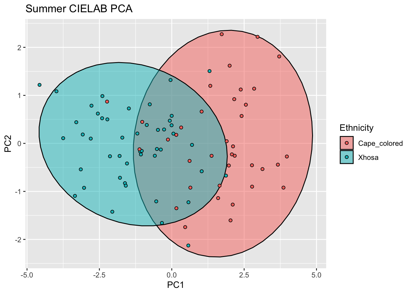
| Version | Author | Date |
|---|---|---|
| e86fbb5 | Lily Heald | 2025-04-04 |
fviz_contrib(summer_cie_pca, choice = "var", axes = 1, top = 10)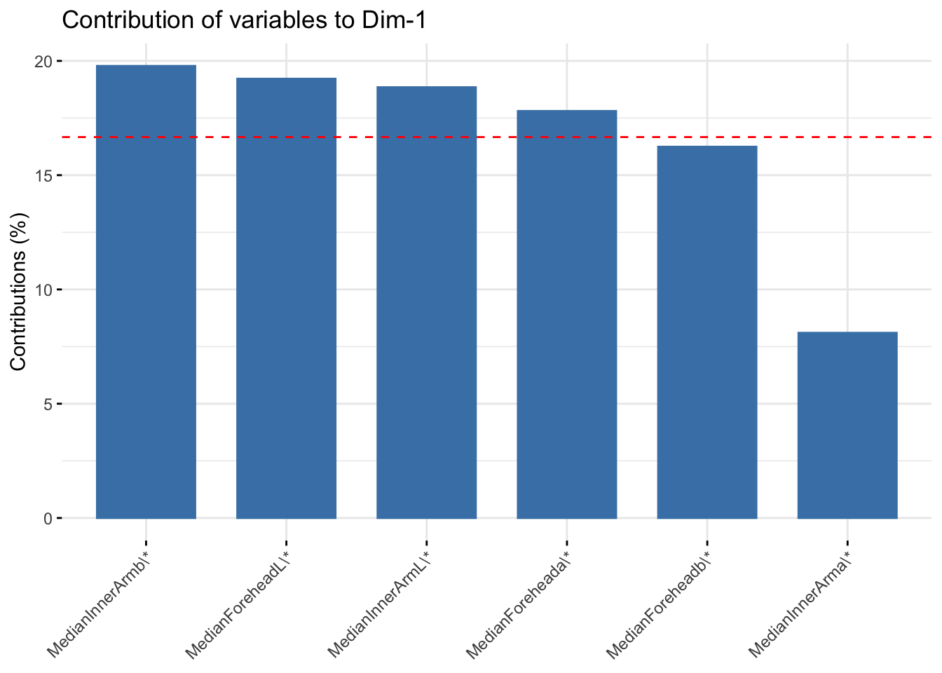
| Version | Author | Date |
|---|---|---|
| e86fbb5 | Lily Heald | 2025-04-04 |
fviz_contrib(summer_cie_pca, choice = "var", axes = 2, top = 10)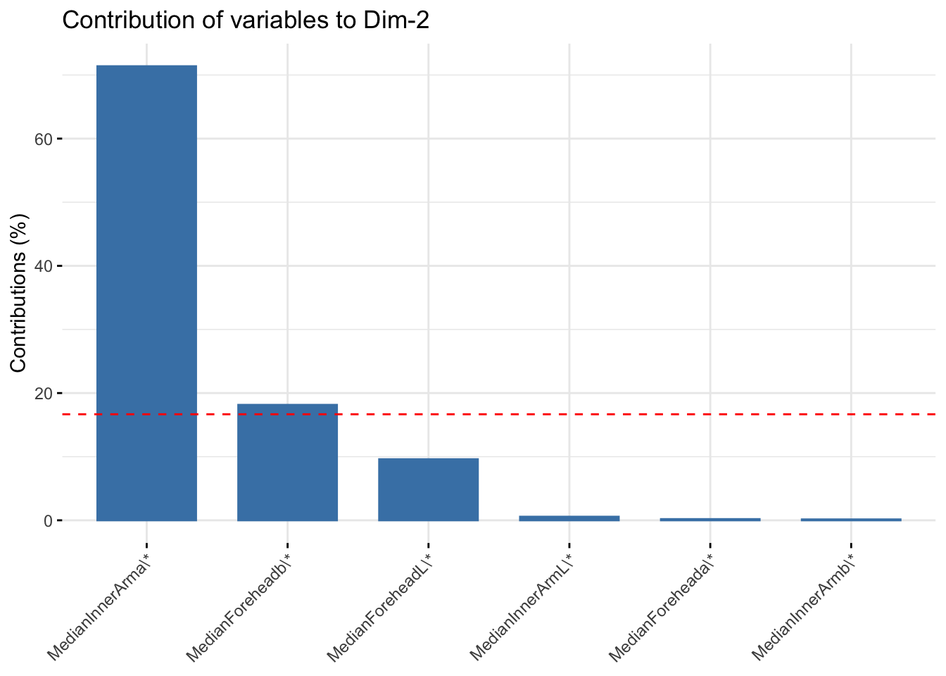
| Version | Author | Date |
|---|---|---|
| e86fbb5 | Lily Heald | 2025-04-04 |
six_cie_scale <- scale(six_cie)
six_cie_pca <- prcomp(six_cie_scale)
summary(six_cie_pca)
Importance of components:
PC1 PC2 PC3 PC4 PC5 PC6
Standard deviation 2.029 1.0710 0.59501 0.50452 0.26435 0.24181
Proportion of Variance 0.686 0.1912 0.05901 0.04242 0.01165 0.00975
Cumulative Proportion 0.686 0.8772 0.93618 0.97861 0.99025 1.00000six_cie_pca$loadings[, 1:2]NULLfviz_eig(six_cie_pca, addlabels = TRUE)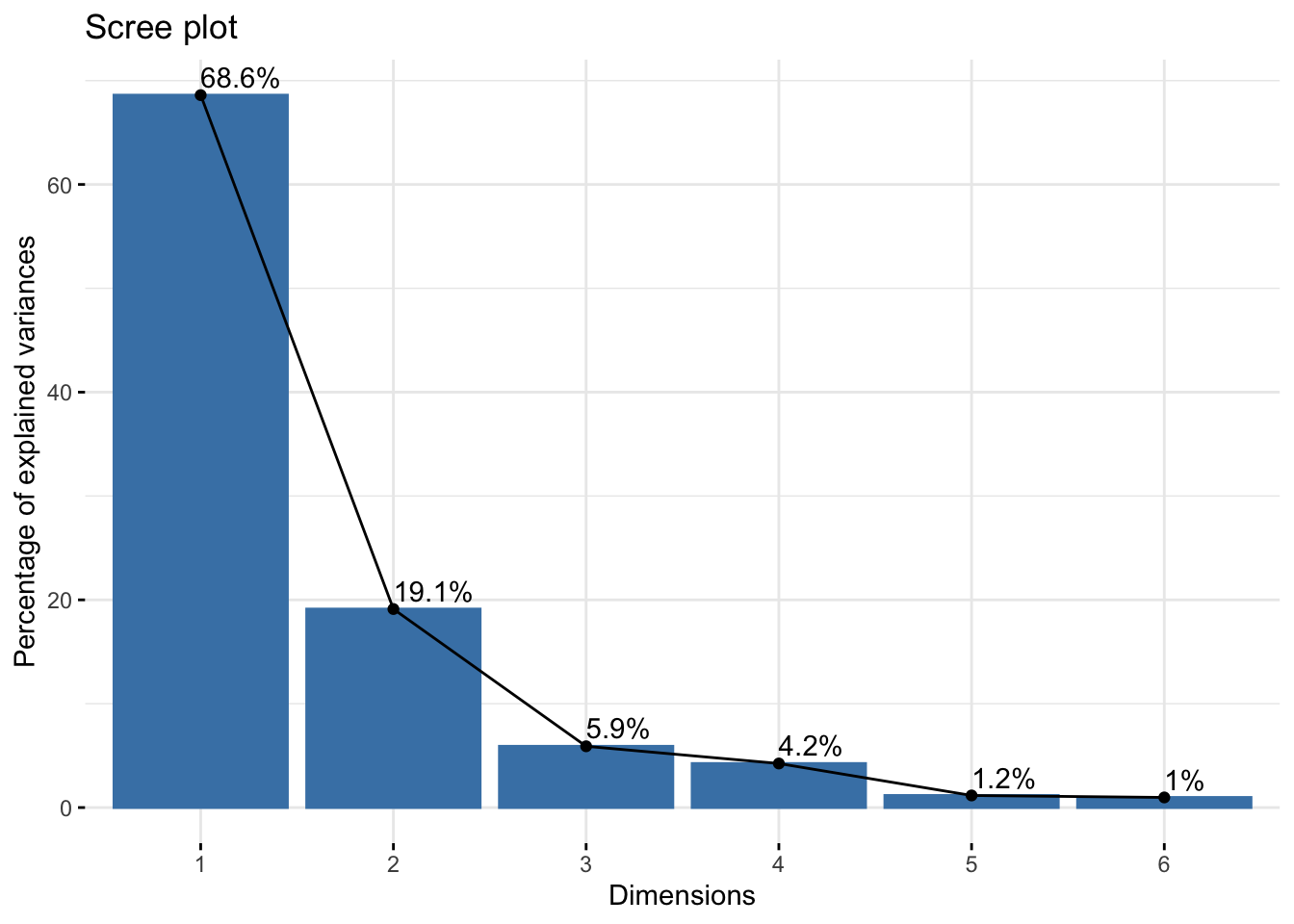
| Version | Author | Date |
|---|---|---|
| e86fbb5 | Lily Heald | 2025-04-04 |
fviz_pca_var(six_cie_pca, col.var = "black")
| Version | Author | Date |
|---|---|---|
| e86fbb5 | Lily Heald | 2025-04-04 |
fviz_cos2(six_cie_pca, choice = "var", axes = 1:2)
| Version | Author | Date |
|---|---|---|
| e86fbb5 | Lily Heald | 2025-04-04 |
six_cie_comps <- as.data.frame(six_cie_pca$x)
six_cie_new <- cbind(six_week_data,six_cie_comps[,c(1,2)])

ggplot(six_rgb_new, aes(x=PC1, y=PC2, col = Ethnicity, fill = Ethnicity)) +
  stat_ellipse(geom = "polygon", col= "black", alpha =0.5)+
  geom_point(shape=21, col="black") +
  labs(title = "Six Week CIELAB PCA")
| Version | Author | Date |
|---|---|---|
| e86fbb5 | Lily Heald | 2025-04-04 |
fviz_contrib(six_cie_pca, choice = "var", axes = 1, top = 10)
| Version | Author | Date |
|---|---|---|
| e86fbb5 | Lily Heald | 2025-04-04 |
fviz_contrib(six_cie_pca, choice = "var", axes = 2, top = 10)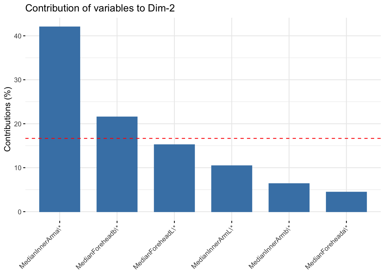
| Version | Author | Date |
|---|---|---|
| e86fbb5 | Lily Heald | 2025-04-04 |
sessionInfo()R version 4.4.2 (2024-10-31)
Platform: aarch64-apple-darwin20
Running under: macOS Monterey 12.5.1
Matrix products: default
BLAS: /Library/Frameworks/R.framework/Versions/4.4-arm64/Resources/lib/libRblas.0.dylib
LAPACK: /Library/Frameworks/R.framework/Versions/4.4-arm64/Resources/lib/libRlapack.dylib; LAPACK version 3.12.0
locale:
[1] en_US.UTF-8/en_US.UTF-8/en_US.UTF-8/C/en_US.UTF-8/en_US.UTF-8
time zone: America/Detroit
tzcode source: internal
attached base packages:
[1] stats graphics grDevices utils datasets methods base
other attached packages:
[1] lme4_1.1-36 Matrix_1.7-2 rstatix_0.7.2 ggpubr_0.6.0
[5] ggfortify_0.4.17 wesanderson_0.3.7 missMDA_1.19 FactoMineR_2.11
[9] factoextra_1.0.7 ggcorrplot_0.1.4.1 corrr_0.4.4 readxl_1.4.3
[13] lubridate_1.9.4 forcats_1.0.0 stringr_1.5.1 purrr_1.0.4
[17] tibble_3.2.1 ggplot2_3.5.1 tidyverse_2.0.0 tidyr_1.3.1
[21] dplyr_1.1.4 readr_2.1.5 workflowr_1.7.1
loaded via a namespace (and not attached):
[1] Rdpack_2.6.2 gridExtra_2.3 sandwich_3.1-1
[4] rlang_1.1.5 magrittr_2.0.3 git2r_0.35.0
[7] multcomp_1.4-28 compiler_4.4.2 getPass_0.2-4
[10] callr_3.7.6 vctrs_0.6.5 pkgconfig_2.0.3
[13] shape_1.4.6.1 fastmap_1.2.0 backports_1.5.0
[16] labeling_0.4.3 utf8_1.2.4 promises_1.3.2
[19] rmarkdown_2.29 tzdb_0.4.0 nloptr_2.1.1
[22] ps_1.9.0 xfun_0.51 glmnet_4.1-8
[25] jomo_2.7-6 cachem_1.1.0 jsonlite_1.9.0
[28] flashClust_1.01-2 later_1.4.1 pan_1.9
[31] broom_1.0.7 parallel_4.4.2 cluster_2.1.8
[34] R6_2.6.1 bslib_0.9.0 stringi_1.8.4
[37] car_3.1-3 rpart_4.1.24 boot_1.3-31
[40] jquerylib_0.1.4 cellranger_1.1.0 estimability_1.5.1
[43] Rcpp_1.0.14 iterators_1.0.14 knitr_1.49
[46] zoo_1.8-12 nnet_7.3-20 httpuv_1.6.15
[49] splines_4.4.2 timechange_0.3.0 tidyselect_1.2.1
[52] abind_1.4-8 rstudioapi_0.17.1 yaml_2.3.10
[55] doParallel_1.0.17 codetools_0.2-20 processx_3.8.5
[58] lattice_0.22-6 withr_3.0.2 coda_0.19-4.1
[61] evaluate_1.0.3 survival_3.8-3 pillar_1.10.1
[64] carData_3.0-5 mice_3.17.0 whisker_0.4.1
[67] DT_0.33 foreach_1.5.2 reformulas_0.4.0
[70] generics_0.1.3 rprojroot_2.0.4 hms_1.1.3
[73] munsell_0.5.1 scales_1.3.0 minqa_1.2.8
[76] xtable_1.8-4 leaps_3.2 glue_1.8.0
[79] emmeans_1.10.7 scatterplot3d_0.3-44 tools_4.4.2
[82] ggsignif_0.6.4 fs_1.6.5 mvtnorm_1.3-3
[85] grid_4.4.2 rbibutils_2.3 colorspace_2.1-1
[88] nlme_3.1-167 Formula_1.2-5 cli_3.6.4
[91] gtable_0.3.6 sass_0.4.9 digest_0.6.37
[94] ggrepel_0.9.6 TH.data_1.1-3 farver_2.1.2
[97] htmlwidgets_1.6.4 htmltools_0.5.8.1 lifecycle_1.0.4
[100] httr_1.4.7 multcompView_0.1-10 mitml_0.4-5
[103] MASS_7.3-64