This reproducible R Markdown
analysis was created with workflowr (version
1.7.1). The Checks tab describes the reproducibility checks
that were applied when the results were created. The Past
versions tab lists the development history.
Great job! The global environment was empty. Objects defined in the
global environment can affect the analysis in your R Markdown file in
unknown ways. For reproduciblity it’s best to always run the code in an
empty environment.
The command set.seed(20230302) was run prior to running
the code in the R Markdown file. Setting a seed ensures that any results
that rely on randomness, e.g. subsampling or permutations, are
reproducible.
Great! You are using Git for version control. Tracking code development
and connecting the code version to the results is critical for
reproducibility.
The results in this page were generated with repository version
35e5bd5.
See the Past versions tab to see a history of the changes made
to the R Markdown and HTML files.
Note that you need to be careful to ensure that all relevant files for
the analysis have been committed to Git prior to generating the results
(you can use wflow_publish or
wflow_git_commit). workflowr only checks the R Markdown
file, but you know if there are other scripts or data files that it
depends on. Below is the status of the Git repository when the results
were generated:
Note that any generated files, e.g. HTML, png, CSS, etc., are not
included in this status report because it is ok for generated content to
have uncommitted changes.
These are the previous versions of the repository in which changes were
made to the R Markdown (analysis/racial_proportion.Rmd) and
HTML (docs/racial_proportion.html) files. If you’ve
configured a remote Git repository (see ?wflow_git_remote),
click on the hyperlinks in the table below to view the files as they
were in that past version.
To analyse the comparison between the M&T forensic DNA database
and census database, we have to attain the racial breakdown (e.g., the
proportions of black, white people) of the state-level forensic database
across the US. However, the breakdown is given in only 7 states, which
are California, Florida, Indiana, Maine, Nevada, South Dakota and Texas.
Thus, we need to develop a statistical model to estimate the proportions
of black and white Americans in the remaining 43 states. Specifically,
we focus on the differences of the racial breakdown between the forensic
database and census database.
2 Binomial Logistic Regression Model
In the underlying work, we establish binomial regression models to
make the estimations. To make the main findings interpretable, we will
give a brief introduction of this common model.
If you don’t care about the details of the binomial regression model,
just feel free to skip this part .
Firstly, we introduces the concept of binomial distributions. Suppose
in each observation, an event has two possible states, success or
failure, and the probability of success is defined as \(p\). Then in \(n\) observations, the number of success
\(y\in \{0,1,\ldots, n\}\) follows a
binomial distribution \(\text{B}(n,p)\). A special case of the
binomial distribution is \(n=1\), where
the distribution is the simple Bernouli distribution. The success
probability \(p\) determines the
characteristics of the binomial distribution. An important property is
that the expectation is given by \(np\).
Now we can delve into the binomial regression. Let the predictor be
\(x\) and the response variable be
\(y\), we assume \[y|x\sim \text{B}(n, g(x^\top \beta)),\]
where \(\beta\) is the coefficients,
and \(g\) is a link function taking
values in \([0,1]\). The popular
choices of \(g\) include Logit and
Probit functions. Here we choose the Logit link function for its
interpretability, which is given by \[g:\mathbb{R}\rightarrow [0,1], \quad
g(z)=\frac{\exp(z)}{\exp(z)+1}.\] To fit this model, we will
estimate the linear coefficients \(\hat{\beta}\), thereby we can predict the
success probability \(\hat{p}=g(x_*^\top
\hat{\beta})\) on a new point \(x_*\), which can be considered as the
proportion of success events given \(x_*\).
3 Data and Model Setting
In this section, we demonstrate the response variable and predictors
used in the binomial regression, and give the concrete model
equation.
3.1 Response variable:
The total number of people for each state in the M&T forensic
database.
The number of each race for each state in the M&T database.
3.2 Predictor:
The proportion of black and white people for each state in the
census database.
The proportion of black and white people of the prison population
for each state.
3.3 Stick-breaking:
We divide the people of the US into three categories, black + white +
other. Then we need to estimate the complete racial breakdown for three
categories in each state. To ensure the sum of these percents is equal
to 1, we use a simple stick-breaking technique. That is, we separately
estimate the percent of white people in all people \(p_{1}\) and the percent of black people in
non-white people \(p_{2}\). Then the
racial breakdown is given by \[\pi_{white}=p_1, \quad
\pi_{black}=(1-p_1)p_2,\quad \pi_{other}=(1-p_1)(1-p_2).\] We run
2 binomial regression models to predict \(p_1\) and \(p_2\) for each state.
3.4 Model equation
Compared to the predictors used by Hanna, we remove the racial
indicator and the interaction between the racial indicator and the
census/prison proportion to avoid colinearity, which leads to a singular
problem for linear regression. Therefore, the model equations are
defined as \[ \frac{white}{all} =
g(\beta_{00} + \beta_{01}*white_{census}+ \beta_{02}*white_{prison}),
\]\[ \frac{black}{nonwhite} =
g(\beta_{10} + \beta_{11}*black_{census} + \beta_{12}*black_{prison}).
\]
3.5 Coefficient interpretability
To interpreter those coefficients, we simply denote the binomial
logistic regression model as \[p = g(\beta_0
+ \sum_{j=1}^p\beta_j x_{j}),\] where \(g\) is the logit link function and \(x_j\) for \(1,\ldots,p\) are covariates. We consider an
odds as \(p/(1-p)\), which is the ratio
of success probabilities versus failure probabilities. Thus, using the
logit link function, the model equation can be written as \[\log(\frac{p}{1-p})=\beta_0 + \sum_{j=1}^p\beta_j
x_{j}.\] Therefore, we can interpreter the coefficients \(\beta_j\) as the increase in the log odds
for every unit increase in \(x_j\).
4 Model Evaluation
If you just want to read the answers to the
key questions, please skip this part and go to the next section
directly.
4.1 Coefficient estimatioan and hypothesis testing
We estimate the linear coefficients \(\beta\) of the binomial logistic regression
for black Americans and white Americans using glm()
function and do a Wald test on the beta coefficients. The \(p\)-values show that these coefficients are
all statistically significant.
Call:
glm(formula = cbind(y[, 1], y[, 3] - y[, 1]) ~ census.percent.white +
    incarc.percent.white, family = binomial, data = train_data)

Coefficients:
                     Estimate Std. Error z value Pr(>|z|)
(Intercept)          -2.89315    0.01097 -263.80   <2e-16 ***
census.percent.white  3.29887    0.03424   96.34   <2e-16 ***
incarc.percent.white  2.17351    0.03143   69.16   <2e-16 ***
---
Signif. codes:  0 '***' 0.001 '**' 0.01 '*' 0.05 '.' 0.1 ' ' 1

(Dispersion parameter for binomial family taken to be 1)

    Null deviance: 599698  on 6  degrees of freedom
Residual deviance:  85204  on 4  degrees of freedom
AIC: 85300

Number of Fisher Scoring iterations: 4
Call:
glm(formula = cbind(y[, 2], y[, 3] - y[, 1] - y[, 2]) ~ census.remain.percent.black +
    incarc.remain.percent.black, family = binomial, data = train_data)

Coefficients:
                             Estimate Std. Error z value Pr(>|z|)
(Intercept)                 -3.923344   0.008174  -480.0   <2e-16 ***
census.remain.percent.black -0.432640   0.027555   -15.7   <2e-16 ***
incarc.remain.percent.black  8.109374   0.032434   250.0   <2e-16 ***
---
Signif. codes:  0 '***' 0.001 '**' 0.01 '*' 0.05 '.' 0.1 ' ' 1

(Dispersion parameter for binomial family taken to be 1)

    Null deviance: 960397  on 6  degrees of freedom
Residual deviance:  29623  on 4  degrees of freedom
AIC: 29710

Number of Fisher Scoring iterations: 4
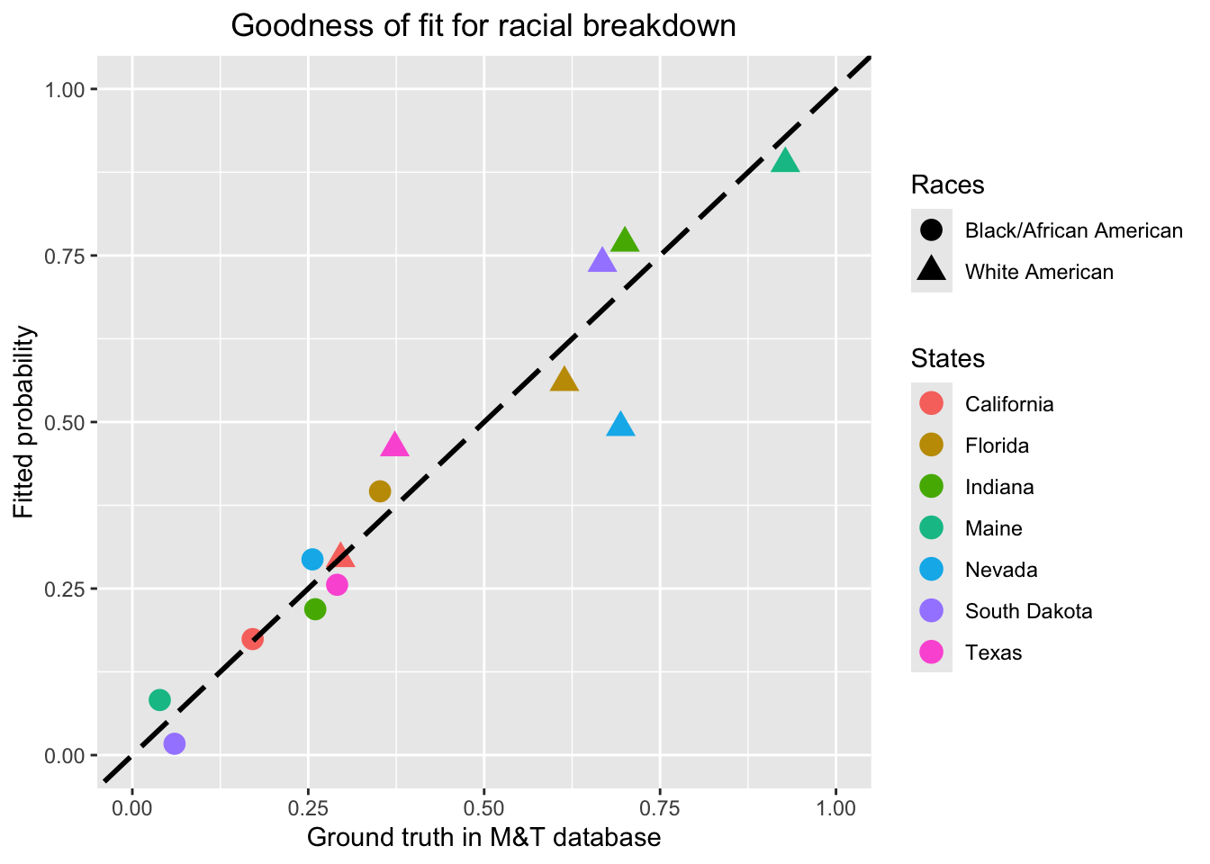
4.2 Goodness-of-Fit
Furthermore, we plot the fitted racial proportions using
stick-breaking binomial regression versus the ground truth for the 7
states with available data. This figure shows that data points are
around the identical map, which means our model fits the training data
well at least.
Black Americans are significantly overrepresented while White
Americans are underrepresented in M&T forensic database compared to
census representation.
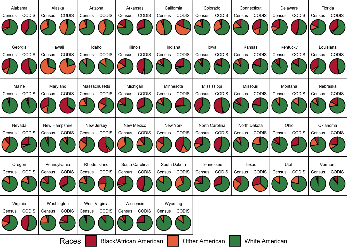
5.2 Racial breakdown
We generate side-by-side pie charts for each state showing the racial
composition according to the census (left) versus the estimated racial
composition of CODIS (right) for each state. From the following figure,
Black/African Americans are overrepresented and white Americans are
underrepresented in CODIS compared to Census.
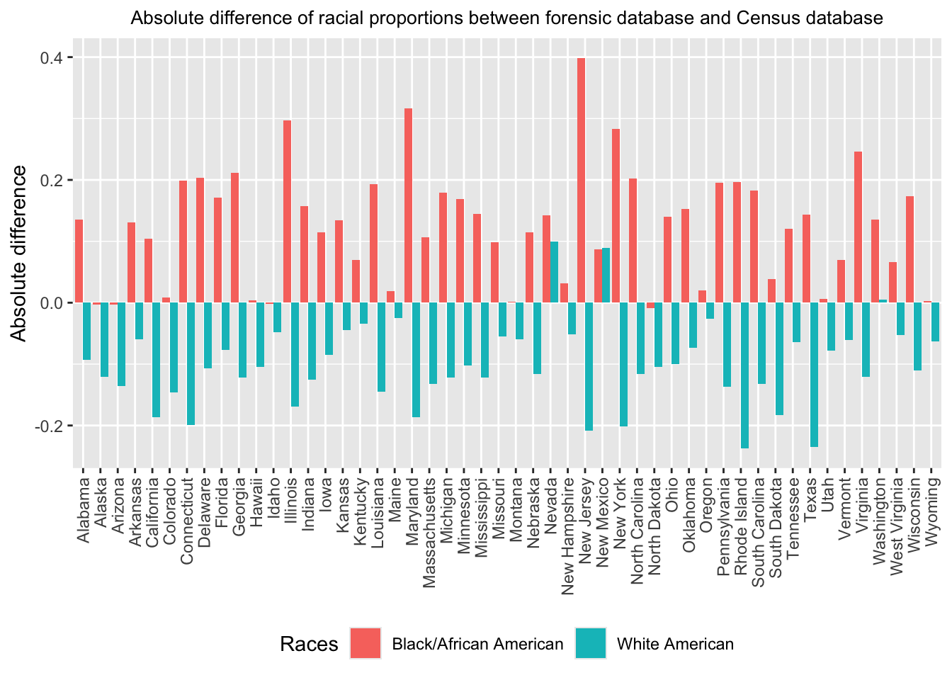
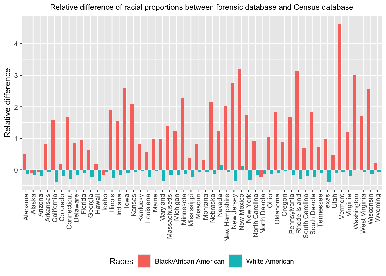
To compare racial proportions between CODIS and Census in each state,
we visualize the absolute differences and relative differences of racial
proportions. These differences are defined as followings, \[\begin{equation*}
\begin{split}
absolute~difference=Proportion_{CODIS}-Proportion_{Census},\\
relative~difference=\frac{Proportion_{CODIS}-Proportion_{Census}}{Proportion_{Census}}.
\end{split}
\end{equation*}\] The difference barcharts show that
Black/African Americans are sigficantly overrepresented in all states
and White Americans are underrepresented in most states in M&T
forensic database compared to census representation.
Based on the asymptotic theory for maximum likelihood estimation, as
the sample size increase, \[\sqrt{n}(\hat{\beta}-\beta) \to N(0, ~
I^{-1}(\beta)),\quad as~n\to \infty,\] where \(I(\beta)\) is the Fisher information. Thus,
the log odds approximately follows the normal distribution, \[\log(\frac{\hat{p}}{1-\hat{p}}) \sim N(x^\top
\beta, ~ \frac{1}{n}x^\top I^{-1}(\beta)x),\] as the total number
of population in 7 states is very large. This normal approximation is
useful in the following hypothesis testing and confidence interval
construction.
For each state, we consider a hypothesis testing problem for the
difference of white proportions between Census and CODIS, \[H_0:p_{CODIS,White}=p_{Census,White}
\leftrightarrow H_1:p_{CODIS,White}>p_{Census,White}.\] Using
the logit link function, we work on the log odds instead of the
probability. The normal approximation helps to construct a one-sided
testing statistics, and the \(p{\text
-values}<10^{-15}\) for all states.
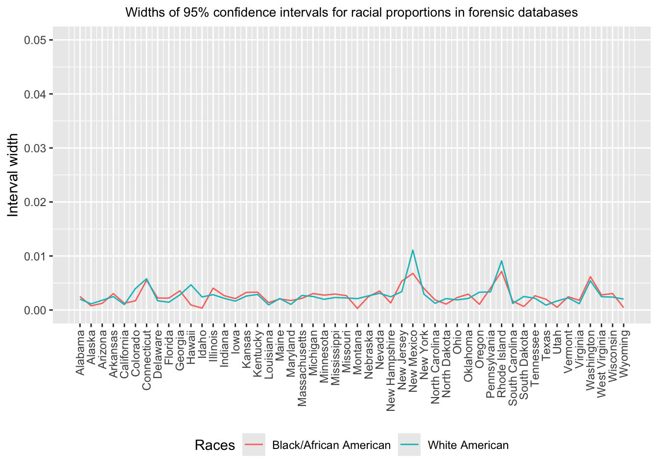
Finally, we calculate the \(1-\alpha\) confidence intervals for the
fitted probability using binomial regression. The normal approximation
for the log odds \(z=x^\top \beta\)
contributes to a confidence interval \(ConfInt=[g(\hat{z}-c_{1-\alpha/2}se(\hat{z})),~g(\hat{z}+c_{1-\alpha/2}se(\hat{z}))]\)
for the white proportion in Census, where \(c_{1-\alpha/2}\) is the \(1-\alpha/2\) quantile of the standard
normal distribution. This implies a confidence interval for the
differences with \(ConfInt-p_{Census}\). For the black
Americans, we utilize a Bonferroni method to construct the confidence
interval. As the number of population in each state with available data
is very large, the estimated standard errors \(se(\hat{z})\) is very small, causing that
the interval widths are almost equal to zero compared to the point
estimation. It also explains why the \(p\)-values for the above hypothesis testing
are nearly zero.