Family structure distribution fitting for genetic surveillance simulations

workflowr

• Summary
• Checks
• Past versions

Last updated: 2025-06-19

Checks: 6 1

Knit directory: PODFRIDGE/

This reproducible R Markdown analysis was created with workflowr (version 1.7.1). The Checks tab describes the reproducibility checks that were applied when the results were created. The Past versions tab lists the development history.

---

R Markdown file: uncommitted changes

The R Markdown file has unstaged changes. To know which version of the R Markdown file created these results, you’ll want to first commit it to the Git repo. If you’re still working on the analysis, you can ignore this warning. When you’re finished, you can run wflow_publish to commit the R Markdown file and build the HTML.

Environment: empty

Great job! The global environment was empty. Objects defined in the global environment can affect the analysis in your R Markdown file in unknown ways. For reproduciblity it’s best to always run the code in an empty environment.

Seed: set.seed(20230302)

The command set.seed(20230302) was run prior to running the code in the R Markdown file. Setting a seed ensures that any results that rely on randomness, e.g. subsampling or permutations, are reproducible.

Session information: recorded

Great job! Recording the operating system, R version, and package versions is critical for reproducibility.

Cache: none

Nice! There were no cached chunks for this analysis, so you can be confident that you successfully produced the results during this run.

File paths: relative

Great job! Using relative paths to the files within your workflowr project makes it easier to run your code on other machines.

Repository version: 7604e1d

Great! You are using Git for version control. Tracking code development and connecting the code version to the results is critical for reproducibility.

The results in this page were generated with repository version 7604e1d. See the Past versions tab to see a history of the changes made to the R Markdown and HTML files.

Note that you need to be careful to ensure that all relevant files for the analysis have been committed to Git prior to generating the results (you can use wflow_publish or wflow_git_commit). workflowr only checks the R Markdown file, but you know if there are other scripts or data files that it depends on. Below is the status of the Git repository when the results were generated:

Ignored files:
    Ignored:    .DS_Store
    Ignored:    .Rhistory
    Ignored:    .Rproj.user/
    Ignored:    data/.DS_Store
    Ignored:    data/sims/.DS_Store
    Ignored:    output/.DS_Store
    Ignored:    output/simulation_20240726-155743/.DS_Store
    Ignored:    output/simulation_20240726-162034_11228488/.DS_Store
    Ignored:    output/simulation_20240726-163235_11228791/.DS_Store

Unstaged changes:
    Modified:   analysis/fertility_assumptions.Rmd

Note that any generated files, e.g. HTML, png, CSS, etc., are not included in this status report because it is ok for generated content to have uncommitted changes.

---

These are the previous versions of the repository in which changes were made to the R Markdown (analysis/fertility_assumptions.Rmd) and HTML (docs/fertility_assumptions.html) files. If you’ve configured a remote Git repository (see ?wflow_git_remote), click on the hyperlinks in the table below to view the files as they were in that past version.

File	Version	Author	Date	Message
Rmd	b9c32a9	Tina Lasisi	2025-06-18	Created fertility assumptions supplementary doc
html	b9c32a9	Tina Lasisi	2025-06-18	Created fertility assumptions supplementary doc

---

U.S. Census Data on Population Differences in Fertility

Here we extract the mean fertility (μ), dispersion/size (θ), and zero‑inflation probability (π₀) for U.S. women aged 50‑59 in the 1990 Census. Women aged 50–59 in the 1990 U.S. Census were born between 1931 and 1940. Assuming a typical childbearing age range of 25–45, their children would have been born between approximately 1956 and 1985. Therefore, the fertility distributions and relative counts estimated from this cohort primarily reflect the family-building behaviors and social contexts of the mid-1950s through the mid-1980s. We filter to Black/African American and White American groups as these are of interest to our paper.

Libraries

library(dplyr)
library(tidyr)
library(readr)
library(MASS)     ## glm.nb
library(pscl)     ## zeroinfl
library(knitr)    ## kable

##knitr::opts_knit$set(root.dir = ".")
knitr::opts_chunk$set(eval = TRUE, echo = TRUE, warning = FALSE, fig.width = 9, fig.height = 7)

Load the pre‑filtered IPUMS subset

path         <- file.path(".", "data")
prop_race_year <- file.path(path, "proportions_table_by_race_year.csv")
data_filter    <- file.path(path, "data_filtered_recoded.csv")

## original script loads both; we only need mother_data for this step
mother_data <- read_csv(data_filter, show_col_types = FALSE)

mother_data already contains:

• YEAR – Census year (1960,1970,1980,1990)
• AGE – respondent age
• RACE – recoded as “White” or “Black/African American”
• chborn_num – completed fertility (children ever born)

Select the 1990, age 50‑59 cohort

cohort <- mother_data %>%
  filter(YEAR == 1990,
         AGE  >= 50, AGE <= 59,
         RACE %in% c("White", "Black/African American")) %>%
  mutate(RACE = droplevels(factor(RACE)))

cohort %>% count(RACE, name = "n_women")

# A tibble: 2 × 2
  RACE                   n_women
  <fct>                    <int>
1 Black/African American   10945
2 White                    96079

Fit Poisson, NB, ZIP, and ZINB per race

fit_four <- function(dat) {
  ## Poisson and NB use standard glm / glm.nb
  pois <- glm(chborn_num ~ 1, family = poisson, data = dat)
  nb   <- glm.nb(chborn_num ~ 1, data = dat)
  
  ## Zero‑inflated models (pscl::zeroinfl)
  zip  <- zeroinfl(chborn_num ~ 1 | 1, data = dat, dist = "poisson")
  zinb <- zeroinfl(chborn_num ~ 1 | 1, data = dat, dist = "negbin")
  
  tibble(
    Model = c("Poisson", "NB", "ZIP", "ZINB"),
    mu    = c(exp(coef(pois)[1]),                    ## log‑link → exp() gives mean
              exp(coef(nb)[1]),
              exp(zip$coefficients$count[1]),        ## intercept of count part
              exp(zinb$coefficients$count[1])),
    size  = c(Inf,                                   ## dispersion θ; Inf = Poisson
              nb$theta,
              Inf,
              zinb$theta),
    pi0   = c(0,                                      ## zero‑inflation prob.
              0,
              plogis(zip$coefficients$zero[1]),
              plogis(zinb$coefficients$zero[1])),
    AIC   = c(AIC(pois), AIC(nb), AIC(zip), AIC(zinb))
  )
}

param_tbl <- cohort %>%
  group_by(RACE) %>%
  group_modify(~ fit_four(.x)) %>%
  ungroup()

Results

knitr::kable(param_tbl, digits = 3,
             caption = "Fertility‑model parameter estimates for women aged50‑59 (1990 Census)")

Fertility‑model parameter estimates for women aged50‑59 (1990 Census)

RACE	Model	mu	size	pi0	AIC
Black/African American	Poisson	3.724	Inf	0.000	55107.97
Black/African American	NB	3.724	3.007	0.000	51184.00
Black/African American	ZIP	4.121	Inf	0.096	52841.82
Black/African American	ZINB	3.932	4.289	0.053	51024.46
White	Poisson	2.895	Inf	0.000	381107.37
White	NB	2.895	18.402	0.000	380052.99
White	ZIP	3.079	Inf	0.060	376840.14
White	ZINB	3.079	257628.938	0.060	376842.17

Table. Fertility-model parameter estimates for women aged 50–59 in the 1990 U.S. Census. Columns are: Model (distribution fitted: Poisson, Negative Binomial [NB], Zero-Inflated Poisson [ZIP], or Zero-Inflated Negative Binomial [ZINB]); μ (mean completed fertility, i.e., average number of children per woman); size (dispersion parameter, only meaningful for NB/ZINB models—set to Inf where not applicable); π₀ (probability of “excess” zeroes, i.e., extra childless women above model expectation, relevant only for ZIP/ZINB models); and AIC (Akaike Information Criterion for model comparison; lower values indicate better fit).

write_csv(param_tbl, "data/fertility_params_1990_50-59.csv")

For women aged 50–59 in the 1990 Census, mean completed fertility (μ) was higher in Black/African American (μ ≈ 3.9, best-fit ZINB) than in White (μ ≈ 3.1, best-fit ZIP) populations. The best-fitting model for Black women was the Zero-Inflated Negative Binomial (ZINB), reflecting both significant overdispersion (θ ≈ 4.3) and a moderate excess of childless women (π₀ ≈ 0.05). For White women, the best fit was the Zero-Inflated Poisson (ZIP), with low overdispersion (θ ≫ 1) and similar zero-inflation (π₀ ≈ 0.06); however, the ZINB model provided a nearly identical fit (ΔAIC < 2), so we use ZINB parameters for both populations in all downstream simulations for consistency and comparability. This approach ensures that our estimates reflect both mean differences and any potential overdispersion or zero inflation in the data for both groups.

Effect of distribution assumptions on relative counts

Here we evaluate how different fertility distribution assumptions (Poisson, Negative Binomial [NB], Zero-Inflated Poisson [ZIP], and Zero-Inflated Negative Binomial [ZINB]) influence estimates of genetically detectable relatives. Using model parameters (param_tbl) previously estimated for each race, we simulate family structures and compare the expected number of siblings, aunts/uncles, and cousins. Grandparents and parents are treated as constants. We present both variable relative counts and totals that include these constants, and provide formal statistical comparisons of distributions. In addition, we compare results to a scenario where the mean number of children is fixed at 2.5 for all distributions.

Calculating the overall mean fertility

For each distribution, we calculate the overall (population-level) mean number of children per woman. For zero-inflated models (ZIP and ZINB), this is calculated as (1 – π₀) × μ, while for Poisson and NB models it is simply μ. This table summarizes the fitted values for each race and model:

param_tbl_total <- param_tbl %>%
  mutate(overall_mean = (1 - pi0) * mu)

knitr::kable(param_tbl_total %>%
  dplyr::select(RACE, Model, mu, pi0, overall_mean), digits = 3,
  caption = "Overall mean fertility by model and race")

Overall mean fertility by model and race

RACE	Model	mu	pi0	overall_mean
Black/African American	Poisson	3.724	0.000	3.724
Black/African American	NB	3.724	0.000	3.724
Black/African American	ZIP	4.121	0.096	3.724
Black/African American	ZINB	3.932	0.053	3.724
White	Poisson	2.895	0.000	2.895
White	NB	2.895	0.000	2.895
White	ZIP	3.079	0.060	2.895
White	ZINB	3.079	0.060	2.895

Simulation function

To estimate how family structure varies across models, we simulate pedigrees using each set of parameters. The function below draws the number of children for grandparents, parents, and aunts/uncles using the given distribution and parameters, then returns the resulting counts of siblings, aunts/uncles, and cousins for 10,000 simulated individuals per model/race.

simulate_relatives <- function(Model, mu, size, pi0,
                               n_sim = 10000,
                               max_kids = 12) {
  draw_kids <- function(n) {
    if      (Model == "Poisson") pmin(rpois(n, mu), max_kids)
    else if (Model == "NB")      pmin(rnbinom(n, size, mu = mu), max_kids)
    else if (Model == "ZIP")     ifelse(runif(n) < pi0, 0L,
                                        pmin(rpois(n, mu), max_kids))
    else if (Model == "ZINB")    ifelse(runif(n) < pi0, 0L,
                                        pmin(rnbinom(n, size, mu = mu), max_kids))
    else stop("Unknown model type")
  }

  grandparent_children <- matrix(draw_kids(4 * n_sim), nrow = n_sim, ncol = 4)
  aunts_uncles <- rowSums(pmax(grandparent_children - 1, 0))

  parent_children <- matrix(draw_kids(2 * n_sim), nrow = n_sim, ncol = 2)
  siblings <- rowSums(pmax(parent_children - 1, 0))

  # FIXED: use vapply, always returns integer vector
  cousins <- vapply(aunts_uncles, function(n)
    if (n == 0) 0L else as.integer(sum(draw_kids(n))),
    integer(1)
  )

  tibble::tibble(
    Siblings    = siblings,
    AuntsUncles = aunts_uncles,
    Cousins     = cousins
  )
}

Scenario 1: Using empirically estimated model means

We first simulate relatives using the best-fit parameters for each model and race, which reflect the true underlying distribution in the data.

library(purrr)
n_sim <- 10000

relative_counts_emp <- param_tbl %>%
  mutate(Scenario = "Empirical mean",
         sim = pmap(list(Model, mu, size, pi0),
                    ~ simulate_relatives(..1, ..2, ..3, ..4, n_sim = n_sim))) %>%
  tidyr::unnest(sim)

Scenario 2: Using a fixed mean of 2.5 for all models

To isolate the impact of model shape from differences in mean fertility, we also simulate each model with a fixed mean of 2.5 children. For ZIP and ZINB, μ is rescaled to ensure (1 – π₀) × μ = 2.5.

param_tbl_fixed <- param_tbl %>%
  mutate(mu = ifelse(pi0 == 0, 2.5, 2.5 / (1 - pi0)))

relative_counts_fix <- param_tbl_fixed %>%
  mutate(Scenario = "Fixed mean 2.5",
         sim = pmap(list(Model, mu, size, pi0),
                    ~ simulate_relatives(..1, ..2, ..3, ..4, n_sim = n_sim))) %>%
  tidyr::unnest(sim)

Combine both scenarios and summarize

We then combine all simulated results and summarize the mean counts for each combination of scenario, model, and race.

relative_counts_both <- bind_rows(relative_counts_emp, relative_counts_fix)
summary_variable <- relative_counts_both %>%
  group_by(Scenario, RACE, Model) %>%
  summarise(across(c(Siblings, AuntsUncles, Cousins), mean), .groups = "drop")

knitr::kable(summary_variable, digits = 2,
             caption = "Expected counts of variable relatives by scenario, model, and race")

Expected counts of variable relatives by scenario, model, and race

Scenario	RACE	Model	Siblings	AuntsUncles	Cousins
Empirical mean	Black/African American	NB	5.52	11.03	40.62
Empirical mean	Black/African American	Poisson	5.50	10.93	40.70
Empirical mean	Black/African American	ZINB	5.62	11.18	41.30
Empirical mean	Black/African American	ZIP	5.69	11.30	42.01
Empirical mean	White	NB	3.88	7.85	22.70
Empirical mean	White	Poisson	3.89	7.76	22.45
Empirical mean	White	ZINB	4.01	8.01	23.22
Empirical mean	White	ZIP	3.99	8.00	23.26
Fixed mean 2.5	Black/African American	NB	3.33	6.68	16.69
Fixed mean 2.5	Black/African American	Poisson	3.15	6.40	15.98
Fixed mean 2.5	Black/African American	ZINB	3.32	6.68	16.68
Fixed mean 2.5	Black/African American	ZIP	3.30	6.58	16.50
Fixed mean 2.5	White	NB	3.20	6.42	16.00
Fixed mean 2.5	White	Poisson	3.18	6.30	15.71
Fixed mean 2.5	White	ZINB	3.23	6.49	16.30
Fixed mean 2.5	White	ZIP	3.26	6.47	16.18

Expected counts including constant relatives

The table below includes the two parents and four grandparents per individual, added to the mean expected number of variable relatives.

summary_total <- summary_variable %>%
  mutate(
    Parents = 2,
    Grandparents = 4,
    Total_1st_2nd = Parents + Grandparents + Siblings + AuntsUncles + Cousins
  ) %>%
  dplyr::select(Scenario, RACE, Model, Parents, Grandparents, Siblings, AuntsUncles, Cousins, Total_1st_2nd)

knitr::kable(summary_total, digits = 2,
             caption = "Expected total counts including constant parents and grandparents")

Expected total counts including constant parents and grandparents

Scenario	RACE	Model	Parents	Grandparents	Siblings	AuntsUncles	Cousins	Total_1st_2nd
Empirical mean	Black/African American	NB	2	4	5.52	11.03	40.62	63.17
Empirical mean	Black/African American	Poisson	2	4	5.50	10.93	40.70	63.14
Empirical mean	Black/African American	ZINB	2	4	5.62	11.18	41.30	64.09
Empirical mean	Black/African American	ZIP	2	4	5.69	11.30	42.01	64.99
Empirical mean	White	NB	2	4	3.88	7.85	22.70	40.44
Empirical mean	White	Poisson	2	4	3.89	7.76	22.45	40.11
Empirical mean	White	ZINB	2	4	4.01	8.01	23.22	41.24
Empirical mean	White	ZIP	2	4	3.99	8.00	23.26	41.25
Fixed mean 2.5	Black/African American	NB	2	4	3.33	6.68	16.69	32.70
Fixed mean 2.5	Black/African American	Poisson	2	4	3.15	6.40	15.98	31.53
Fixed mean 2.5	Black/African American	ZINB	2	4	3.32	6.68	16.68	32.68
Fixed mean 2.5	Black/African American	ZIP	2	4	3.30	6.58	16.50	32.38
Fixed mean 2.5	White	NB	2	4	3.20	6.42	16.00	31.63
Fixed mean 2.5	White	Poisson	2	4	3.18	6.30	15.71	31.20
Fixed mean 2.5	White	ZINB	2	4	3.23	6.49	16.30	32.03
Fixed mean 2.5	White	ZIP	2	4	3.26	6.47	16.18	31.91

Visualization: Comparing models and mean specification

We visualize the full distribution of simulated relatives across models, mean scenarios, and races. Each box represents the distribution of simulated counts; means are shown as white dots.

library(ggplot2)

rel_long_all <- relative_counts_both %>%
  tidyr::pivot_longer(c(Siblings, AuntsUncles, Cousins),
                      names_to = "Relative",
                      values_to = "Count") %>%
  mutate(
    Model      = factor(Model, levels = c("Poisson", "ZIP", "NB", "ZINB")),
    Relative   = factor(Relative, levels = c("Siblings","AuntsUncles","Cousins")),
    Scenario   = factor(Scenario, levels = c("Empirical mean","Fixed mean 2.5")),
    RACE       = factor(RACE,    levels = c("Black/African American","White"))
  )

ggplot(rel_long_all,
       aes(x = Model, y = Count, fill = Relative)) +
  geom_boxplot(position = position_dodge(width = 0.8),
               width = 0.7, alpha = .8, outlier.size = .3) +
  stat_summary(fun = mean, geom = "point", shape = 21, size = 1.4,
               aes(group = Relative),
               position = position_dodge(width = 0.8),
               colour = "black", fill = "white") +
  facet_grid(Scenario ~ RACE) +
  scale_fill_viridis_d(option = "D") +
  labs(title   = "Distribution of simulated relatives by model, mean assumption and race",
       x       = "Fertility model",
       y       = "Relative count",
       fill    = "Relative type") +
  theme_minimal(base_size = 11) +
  theme(legend.position = "top",
        axis.title.x    = element_text(vjust = -0.2),
        strip.text      = element_text(size = 10))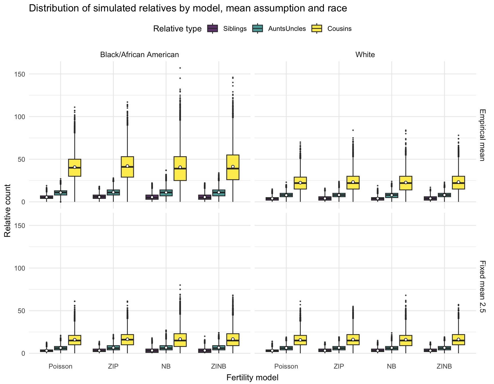

Past versions of unnamed-chunk-7-1.png

Version	Author	Date
b9c32a9	Tina Lasisi	2025-06-18

Statistical modeling: Effects of model, scenario, and their interaction

We formally test the contribution of model choice, mean specification, and race on the simulated number of relatives, using three-way ANOVA for each relative type. We also generate a compact-letter display (CLD) to indicate which groups are or are not statistically different after correction for multiple comparisons. In the summary plot, each box is labeled with its CLD group letter: boxes sharing a letter are not significantly different at the 0.05 level (Bonferroni-adjusted).

library(broom)
library(knitr)

relatives <- c("Siblings", "AuntsUncles", "Cousins")

for (rel in relatives) {
  cat("\n\n### Model for", rel, "\n\n")
  
  analysis_data <- rel_long_all %>%
    mutate(
      RACE = factor(RACE, levels = c("White", "Black/African American")),
      Model = factor(Model, levels = c("Poisson", "ZIP", "NB", "ZINB")),
      Scenario = factor(Scenario, levels = c("Fixed mean 2.5", "Empirical mean")),
      Relative = factor(Relative, levels = c("Siblings", "AuntsUncles", "Cousins"))
    ) %>%
    filter(Relative == rel)
  
  lm_fit <- lm(Count ~ RACE * Model * Scenario, data = analysis_data)
  lm_tidy <- broom::tidy(lm_fit, conf.int = TRUE)
  
  print(knitr::kable(
    lm_tidy,
    digits = 3,
    caption = paste("Regression coefficients for", rel, 
                    "(reference: White, Poisson, Fixed mean 2.5)")
  ))
}

Model for Siblings

Regression coefficients for Siblings (reference: White, Poisson, Fixed mean 2.5)

term	estimate	std.error	statistic	p.value	conf.low	conf.high
(Intercept)	3.184	0.026	121.692	0.000	3.133	3.235
RACEBlack/African American	-0.039	0.037	-1.049	0.294	-0.111	0.034
ModelZIP	0.079	0.037	2.130	0.033	0.006	0.151
ModelNB	0.017	0.037	0.468	0.640	-0.055	0.090
ModelZINB	0.043	0.037	1.176	0.240	-0.029	0.116
ScenarioEmpirical mean	0.706	0.037	19.078	0.000	0.633	0.778
RACEBlack/African American:ModelZIP	0.075	0.052	1.426	0.154	-0.028	0.177
RACEBlack/African American:ModelNB	0.168	0.052	3.211	0.001	0.065	0.271
RACEBlack/African American:ModelZINB	0.127	0.052	2.437	0.015	0.025	0.230
RACEBlack/African American:ScenarioEmpirical mean	1.653	0.052	31.586	0.000	1.550	1.755
ModelZIP:ScenarioEmpirical mean	0.020	0.052	0.382	0.702	-0.083	0.123
ModelNB:ScenarioEmpirical mean	-0.023	0.052	-0.436	0.663	-0.125	0.080
ModelZINB:ScenarioEmpirical mean	0.076	0.052	1.460	0.144	-0.026	0.179
RACEBlack/African American:ModelZIP:ScenarioEmpirical mean	0.008	0.074	0.115	0.909	-0.137	0.154
RACEBlack/African American:ModelNB:ScenarioEmpirical mean	-0.145	0.074	-1.962	0.050	-0.290	0.000
RACEBlack/African American:ModelZINB:ScenarioEmpirical mean	-0.134	0.074	-1.812	0.070	-0.279	0.011

Model for AuntsUncles

Regression coefficients for AuntsUncles (reference: White, Poisson, Fixed mean 2.5)

term	estimate	std.error	statistic	p.value	conf.low	conf.high
(Intercept)	6.301	0.037	170.397	0.000	6.229	6.374
RACEBlack/African American	0.097	0.052	1.860	0.063	-0.005	0.200
ModelZIP	0.165	0.052	3.147	0.002	0.062	0.267
ModelNB	0.122	0.052	2.331	0.020	0.019	0.224
ModelZINB	0.192	0.052	3.681	0.000	0.090	0.295
ScenarioEmpirical mean	1.464	0.052	27.984	0.000	1.361	1.566
RACEBlack/African American:ModelZIP	0.019	0.074	0.254	0.799	-0.126	0.164
RACEBlack/African American:ModelNB	0.164	0.074	2.221	0.026	0.019	0.309
RACEBlack/African American:ModelZINB	0.094	0.074	1.268	0.205	-0.051	0.239
RACEBlack/African American:ScenarioEmpirical mean	3.071	0.074	41.523	0.000	2.926	3.216
ModelZIP:ScenarioEmpirical mean	0.075	0.074	1.009	0.313	-0.070	0.220
ModelNB:ScenarioEmpirical mean	-0.035	0.074	-0.473	0.636	-0.180	0.110
ModelZINB:ScenarioEmpirical mean	0.054	0.074	0.734	0.463	-0.091	0.199
RACEBlack/African American:ModelZIP:ScenarioEmpirical mean	0.107	0.105	1.022	0.307	-0.098	0.312
RACEBlack/African American:ModelNB:ScenarioEmpirical mean	-0.159	0.105	-1.516	0.129	-0.364	0.046
RACEBlack/African American:ModelZINB:ScenarioEmpirical mean	-0.099	0.105	-0.942	0.346	-0.304	0.107

Model for Cousins

Regression coefficients for Cousins (reference: White, Poisson, Fixed mean 2.5)

term	estimate	std.error	statistic	p.value	conf.low	conf.high
(Intercept)	15.713	0.128	122.316	0.000	15.461	15.965
RACEBlack/African American	0.270	0.182	1.487	0.137	-0.086	0.626
ModelZIP	0.467	0.182	2.570	0.010	0.111	0.823
ModelNB	0.291	0.182	1.601	0.109	-0.065	0.647
ModelZINB	0.591	0.182	3.256	0.001	0.235	0.948
ScenarioEmpirical mean	6.739	0.182	37.092	0.000	6.383	7.095
RACEBlack/African American:ModelZIP	0.048	0.257	0.185	0.853	-0.456	0.551
RACEBlack/African American:ModelNB	0.412	0.257	1.606	0.108	-0.091	0.916
RACEBlack/African American:ModelZINB	0.107	0.257	0.415	0.678	-0.397	0.610
RACEBlack/African American:ScenarioEmpirical mean	17.978	0.257	69.974	0.000	17.474	18.481
ModelZIP:ScenarioEmpirical mean	0.337	0.257	1.312	0.189	-0.166	0.841
ModelNB:ScenarioEmpirical mean	-0.037	0.257	-0.145	0.885	-0.541	0.466
ModelZINB:ScenarioEmpirical mean	0.174	0.257	0.677	0.498	-0.330	0.677
RACEBlack/African American:ModelZIP:ScenarioEmpirical mean	0.456	0.363	1.256	0.209	-0.256	1.169
RACEBlack/African American:ModelNB:ScenarioEmpirical mean	-0.746	0.363	-2.054	0.040	-1.459	-0.034
RACEBlack/African American:ModelZINB:ScenarioEmpirical mean	-0.275	0.363	-0.756	0.450	-0.987	0.438

library(dplyr)
library(broom)
library(tidyr)
library(purrr)

relatives <- c("Siblings", "AuntsUncles", "Cousins")
models <- c("Poisson", "ZIP", "NB", "ZINB")

anova_per_model <- purrr::cross_df(list(Relative = relatives, Model = models)) %>%
  rowwise() %>%
  mutate(
    anova = list({
      data_fixed <- rel_long_all %>%
        filter(Relative == Relative, Scenario == "Fixed mean 2.5", Model == Model) %>%
        mutate(RACE = factor(RACE, levels = c("White", "Black/African American")))
      if(nrow(data_fixed) < 2) return(tibble(Df = NA, F_value = NA, p_value = NA))
      lm0 <- lm(Count ~ 1, data = data_fixed)
      lm1 <- lm(Count ~ RACE, data = data_fixed)
      atab <- as.data.frame(anova(lm0, lm1))
      tibble(Df = atab$Df[2], F_value = atab$`F value`[2], p_value = atab$`Pr(>F)`[2])
    })
  ) %>%
  unnest(anova)

knitr::kable(anova_per_model, digits = 4, caption = "Test of Race effect within each model (Fixed mean = 2.5 only)")

Test of Race effect within each model (Fixed mean = 2.5 only)

Relative	Model	Df	p_value
Siblings	Poisson	1	0
AuntsUncles	Poisson	1	0
Cousins	Poisson	1	0
Siblings	ZIP	1	0
AuntsUncles	ZIP	1	0
Cousins	ZIP	1	0
Siblings	NB	1	0
AuntsUncles	NB	1	0
Cousins	NB	1	0
Siblings	ZINB	1	0
AuntsUncles	ZINB	1	0
Cousins	ZINB	1	0

Summary

When mean fertility is held constant at 2.5 children for both populations, the expected number of siblings, aunts/uncles, and cousins is virtually identical for Black and White groups, regardless of model choice (Poisson, NB, ZIP, or ZINB). Although our fitted NB/ZINB/ZIP models allow for group-specific overdispersion and zero-inflation, these parameters had negligible practical effect on expected kin counts for the distributions observed in US Census data. We conclude that, in practice, mean fertility is the primary driver of group differences in simulated kinship structure for recent cohorts.

Individual-Level Sibling Distribution and Kinship Risk

We now assess close-kin counts (siblings, aunts/uncles, cousins) directly from the perspective of the focal individual, fitting and simulating the distribution of siblings per person, and comparing the effect of distributional assumptions (Poisson, NB, ZIP, ZINB) and race, as before.

Fit models to individual-level sibling counts

# Prepare individual-level sibling count
sibs_long <- cohort %>%
  filter(chborn_num > 0) %>%
  tidyr::uncount(chborn_num, .remove = FALSE) %>%
  mutate(n_sib = chborn_num - 1)

fit_sib_models <- function(dat) {
  pois <- glm(n_sib ~ 1, family = poisson, data = dat)
  nb   <- glm.nb(n_sib ~ 1, data = dat)
  zip  <- zeroinfl(n_sib ~ 1 | 1, data = dat, dist = "poisson")
  zinb <- zeroinfl(n_sib ~ 1 | 1, data = dat, dist = "negbin")
  tibble(
    Model = c("Poisson", "NB", "ZIP", "ZINB"),
    mu    = c(exp(coef(pois)[1]),
              exp(coef(nb)[1]),
              exp(zip$coefficients$count[1]),
              exp(zinb$coefficients$count[1])),
    size  = c(Inf, nb$theta, Inf, zinb$theta),
    pi0   = c(0, 0, plogis(zip$coefficients$zero[1]), plogis(zinb$coefficients$zero[1])),
    AIC   = c(AIC(pois), AIC(nb), AIC(zip), AIC(zinb))
  )
}
sib_param_tbl <- sibs_long %>%
  group_by(RACE) %>%
  group_modify(~ fit_sib_models(.x)) %>%
  ungroup()
knitr::kable(sib_param_tbl, digits = 3, caption = "Model fits for sibling count distribution by race")

Model fits for sibling count distribution by race

RACE	Model	mu	size	pi0	AIC
Black/African American	Poisson	4.803	Inf	0.000	203758.5
Black/African American	NB	4.803	6.474000e+00	0.000	197096.3
Black/African American	ZIP	4.930	Inf	0.026	201893.1
Black/African American	ZINB	4.930	2.100902e+09	0.026	201895.1
White	Poisson	3.053	Inf	0.000	1104146.8
White	NB	3.053	1.837100e+01	0.000	1100190.5
White	ZIP	3.053	Inf	0.000	1104149.3
White	ZINB	3.053	6.323171e+10	0.000	1104150.8

Table. For individual-level sibling counts, the negative binomial (NB) model provides the best fit for both populations, with substantially lower AIC than the Poisson, ZIP, or ZINB models. This indicates that sibship size is more variable than would be expected under a simple Poisson process, consistent with substantial overdispersion in family sizes, but there is little evidence for zero-inflation (excess of only children).

Because individuals from large families are more common in an individual-level sample, the average number of siblings per person is higher than the mean family size minus one (the “sibship size paradox”). This effect is important to account for in forensic or genetic risk models that simulate from the perspective of a random individual.

Simulate kin counts for the focal individual

We estimate the expected number and full probability distributions of close genetic relatives (siblings, aunts/uncles, and cousins) for a focal individual. This is done across all fitted models (Poisson, NB, ZIP, ZINB), for both Black/African American and White groups, using both empirical mean and fixed mean scenarios. We then compare these focal-individual predictions to a hybrid “best-fit” model and a Poisson-fertility baseline.

simulate_focal_kin <- function(
  sib_Model, sib_mu, sib_size, sib_pi0,      # Sibling distribution params
  fert_Model, fert_mu, fert_size, fert_pi0,  # Fertility distribution params
  n_sim = 10000, max_sib = 12, max_kids = 12
) {
  # Helper: draw siblings under a distribution (always return integer)
  draw_sibs <- function(nn) {
    out <- if      (sib_Model == "Poisson") rpois(nn, sib_mu)
           else if (sib_Model == "NB")      rnbinom(nn, sib_size, mu = sib_mu)
           else if (sib_Model == "ZIP")     ifelse(runif(nn) < sib_pi0, 0L, rpois(nn, sib_mu))
           else if (sib_Model == "ZINB")    ifelse(runif(nn) < sib_pi0, 0L, rnbinom(nn, sib_size, mu = sib_mu))
           else stop("Unknown sib_model")
    as.integer(pmin(out, max_sib))
  }
  draw_fert <- function(nn) {
    out <- if      (fert_Model == "Poisson") rpois(nn, fert_mu)
           else if (fert_Model == "NB")      rnbinom(nn, fert_size, mu = fert_mu)
           else if (fert_Model == "ZIP")     ifelse(runif(nn) < fert_pi0, 0L, rpois(nn, fert_mu))
           else if (fert_Model == "ZINB")    ifelse(runif(nn) < fert_pi0, 0L, rnbinom(nn, fert_size, mu = fert_mu))
           else stop("Unknown fert_model")
    as.integer(pmin(out, max_kids))
  }

  # 1. Siblings for the focal individual
  siblings <- draw_sibs(n_sim)

  # 2. Aunts & uncles (no subtraction needed)
  aunts_maternal <- draw_sibs(n_sim)   # mother’s siblings
  aunts_paternal <- draw_sibs(n_sim)   # father’s siblings
  aunts_uncles   <- aunts_maternal + aunts_paternal


  # 3. Cousins: for each aunt/uncle, simulate their fertility and sum
  cousins <- purrr::map_int(aunts_uncles, function(n_au) {
    if (n_au == 0L) 0L else as.integer(sum(draw_fert(n_au)))
  })

  tibble::tibble(
    Siblings    = siblings,
    AuntsUncles = aunts_uncles,
    Cousins     = cousins,
    Parents     = 2L,
    Grandparents= 4L,
    TotalKin = siblings + aunts_uncles + cousins + 2 + 4
  )
}

Prepare Parameter Tables

# Sibling (focal individual) parameter tables: empirical and fixed mean scenarios
sib_param_tbl_exp <- sib_param_tbl %>%
  rename(sib_Model = Model, sib_mu = mu, sib_size = size, sib_pi0 = pi0, sib_AIC = AIC)

sib_param_tbl_fixed <- sib_param_tbl %>%
  mutate(sib_mu = ifelse(pi0 == 0, 1.5, 1.5 / (1 - pi0))) %>%
  rename(sib_Model = Model, sib_size = size, sib_pi0 = pi0, sib_AIC = AIC)

# Fertility (collateral relatives) parameter tables: empirical and fixed mean scenarios
fert_param_tbl_exp <- param_tbl %>%
  rename(fert_Model = Model, fert_mu = mu, fert_size = size, fert_pi0 = pi0, fert_AIC = AIC)

fert_param_tbl_fixed <- param_tbl %>%
  mutate(fert_mu = ifelse(pi0 == 0, 2.5, 2.5 / (1 - pi0))) %>%
  rename(fert_Model = Model, fert_size = size, fert_pi0 = pi0, fert_AIC = AIC)

Create Parameter Pairings and Run Simulations

# Parameter pairings for each scenario (all RACE x Model combinations)
param_pairs_emp <- expand_grid(
  RACE = unique(sib_param_tbl_exp$RACE),
  Model = unique(sib_param_tbl_exp$sib_Model)
) %>%
  left_join(sib_param_tbl_exp, by = c("RACE", "Model" = "sib_Model")) %>%
  left_join(fert_param_tbl_exp, by = c("RACE", "Model" = "fert_Model"))

param_pairs_fixed <- expand_grid(
  RACE = unique(sib_param_tbl_fixed$RACE),
  Model = unique(sib_param_tbl_fixed$sib_Model)
) %>%
  left_join(sib_param_tbl_fixed, by = c("RACE", "Model" = "sib_Model")) %>%
  left_join(fert_param_tbl_fixed, by = c("RACE", "Model" = "fert_Model"))

# Simulate kin counts for all parameter combinations (empirical and fixed mean)
focal_kin_sim_results_emp <- param_pairs_emp %>%
  mutate(
    sim = pmap(
      list(Model, sib_mu, sib_size, sib_pi0, fert_mu, fert_size, fert_pi0),
      ~ simulate_focal_kin(
        sib_Model = ..1, sib_mu = ..2, sib_size = ..3, sib_pi0 = ..4,
        fert_Model = ..1, fert_mu = ..5, fert_size = ..6, fert_pi0 = ..7,
        n_sim = 10000
      )
    )
  )

focal_kin_sim_results_fixed <- param_pairs_fixed %>%
  mutate(
    sim = pmap(
      list(Model, sib_mu, sib_size, sib_pi0, fert_mu, fert_size, fert_pi0),
      ~ simulate_focal_kin(
        sib_Model = ..1, sib_mu = ..2, sib_size = ..3, sib_pi0 = ..4,
        fert_Model = ..1, fert_mu = ..5, fert_size = ..6, fert_pi0 = ..7,
        n_sim = 10000
      )
    )
  )

Tidy Results and Label Scenarios

# Unnest and label scenario
focal_kin_counts_emp   <- focal_kin_sim_results_emp   %>% mutate(Scenario = "Empirical mean") %>% unnest(sim)
focal_kin_counts_fixed <- focal_kin_sim_results_fixed %>% mutate(Scenario = "Fixed mean")    %>% unnest(sim)

# Combine for downstream comparison
focal_kin_counts_all <- bind_rows(focal_kin_counts_emp, focal_kin_counts_fixed)

Summarize Mean Kin Counts

summary_focal_kin_all <- focal_kin_counts_all %>%
  group_by(Scenario, RACE, Model) %>%
  summarise(
    mean_sibs         = mean(Siblings),
    mean_aunts_uncles = mean(AuntsUncles),
    mean_cousins      = mean(Cousins),
    mean_total        = mean(TotalKin),
    .groups = "drop"
  )

knitr::kable(summary_focal_kin_all, digits = 2,
             caption = "Expected number of first-, second-, and third-degree relatives for a focal individual (simulated, by model, scenario, and race)")

Expected number of first-, second-, and third-degree relatives for a focal individual (simulated, by model, scenario, and race)

Scenario	RACE	Model	mean_sibs	mean_aunts_uncles	mean_cousins	mean_total
Empirical mean	Black/African American	NB	4.74	9.62	35.68	56.03
Empirical mean	Black/African American	Poisson	4.77	9.59	35.83	56.20
Empirical mean	Black/African American	ZINB	4.80	9.65	35.66	56.12
Empirical mean	Black/African American	ZIP	4.78	9.59	35.65	56.02
Empirical mean	White	NB	3.08	6.11	17.67	32.86
Empirical mean	White	Poisson	3.09	6.15	17.81	33.04
Empirical mean	White	ZINB	3.07	6.14	17.85	33.06
Empirical mean	White	ZIP	3.04	6.08	17.58	32.70
Fixed mean	Black/African American	NB	1.51	2.97	7.41	17.89
Fixed mean	Black/African American	Poisson	1.51	2.99	7.42	17.92
Fixed mean	Black/African American	ZINB	1.50	3.02	7.60	18.13
Fixed mean	Black/African American	ZIP	1.52	3.00	7.50	18.02
Fixed mean	White	NB	1.49	3.00	7.52	18.02
Fixed mean	White	Poisson	1.49	2.99	7.48	17.95
Fixed mean	White	ZINB	1.53	3.01	7.54	18.08
Fixed mean	White	ZIP	1.52	3.00	7.52	18.04

Visualize the Simulated Distributions

# Pivot for plotting
focal_kin_long <- focal_kin_counts_all %>%
  pivot_longer(c(Siblings, AuntsUncles, Cousins),
               names_to = "RelativeType", values_to = "Count") %>%
  mutate(
    Model = factor(Model, levels = c("Poisson", "NB", "ZIP", "ZINB")),
    RelativeType = factor(RelativeType, levels = c("Siblings", "AuntsUncles", "Cousins")),
    RACE = factor(RACE, levels = c("Black/African American", "White"))
  )

# Plot
library(ggplot2)
ggplot(focal_kin_long,
       aes(x = Model, y = Count, fill = RelativeType)) +
  geom_boxplot(position = position_dodge(width = 0.8),
               width = 0.7, alpha = .8, outlier.size = .3) +
  stat_summary(fun = mean, geom = "point", shape = 21, size = 1.4,
               aes(group = RelativeType),
               position = position_dodge(width = 0.8),
               colour = "black", fill = "white") +
  facet_grid(Scenario ~ RACE) +
  scale_fill_viridis_d(option = "D") +
  labs(title   = "Simulated number of close relatives for a focal individual",
       x       = "Sibling-count model",
       y       = "Relative count",
       fill    = "Relative type") +
  theme_minimal(base_size = 11) +
  theme(legend.position = "top")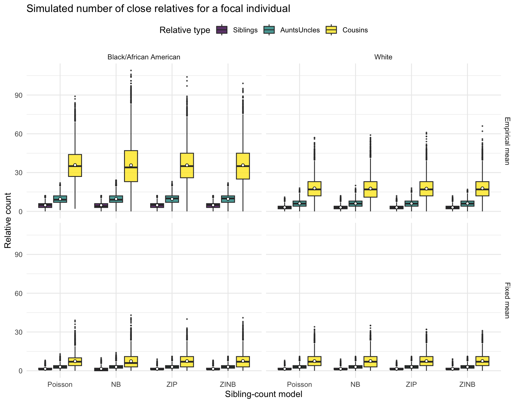

Past versions of unnamed-chunk-14-1.png

Version	Author	Date
b9c32a9	Tina Lasisi	2025-06-18

Regression Models Comparing Scenarios, Models, and Groups

library(broom)
library(knitr)

relatives <- c("Siblings", "AuntsUncles", "Cousins")

for (rel in relatives) {
  cat("\n\n### Focal-individual model for", rel, "\n\n")
  analysis_data <- focal_kin_long %>%
    filter(RelativeType == rel) %>%
    mutate(
      RACE     = factor(RACE, levels = c("White", "Black/African American")),   # White as reference
      Model    = factor(Model, levels = c("Poisson", "NB", "ZIP", "ZINB")),    # Poisson as reference
      Scenario = factor(Scenario, levels = c("Fixed mean", "Empirical mean"))   # Fixed mean as reference
    )
  lm_fit <- lm(Count ~ RACE * Model * Scenario, data = analysis_data)
  lm_tidy <- broom::tidy(lm_fit, conf.int = TRUE)
  print(knitr::kable(
    lm_tidy,
    digits = 3,
    caption = paste(
      "Regression coefficients for", rel, 
      "(focal-individual, reference: White, Poisson, Fixed mean\nSib mean=1.5, Fertility mean=2.5)"
    )
  ))
}

Focal-individual model for Siblings

Regression coefficients for Siblings (focal-individual, reference: White, Poisson, Fixed mean Sib mean=1.5, Fertility mean=2.5)

term	estimate	std.error	statistic	p.value	conf.low	conf.high
(Intercept)	1.491	0.017	85.741	0.000	1.457	1.525
RACEBlack/African American	0.020	0.025	0.825	0.409	-0.028	0.069
ModelNB	0.002	0.025	0.069	0.945	-0.047	0.050
ModelZIP	0.024	0.025	0.984	0.325	-0.024	0.072
ModelZINB	0.038	0.025	1.537	0.124	-0.010	0.086
ScenarioEmpirical mean	1.597	0.025	64.917	0.000	1.549	1.645
RACEBlack/African American:ModelNB	-0.008	0.035	-0.227	0.820	-0.076	0.060
RACEBlack/African American:ModelZIP	-0.020	0.035	-0.561	0.575	-0.088	0.049
RACEBlack/African American:ModelZINB	-0.045	0.035	-1.288	0.198	-0.113	0.023
RACEBlack/African American:ScenarioEmpirical mean	1.661	0.035	47.757	0.000	1.593	1.730
ModelNB:ScenarioEmpirical mean	-0.010	0.035	-0.276	0.783	-0.078	0.059
ModelZIP:ScenarioEmpirical mean	-0.071	0.035	-2.044	0.041	-0.139	-0.003
ModelZINB:ScenarioEmpirical mean	-0.052	0.035	-1.503	0.133	-0.120	0.016
RACEBlack/African American:ModelNB:ScenarioEmpirical mean	-0.014	0.049	-0.293	0.770	-0.111	0.082
RACEBlack/African American:ModelZIP:ScenarioEmpirical mean	0.076	0.049	1.541	0.123	-0.021	0.172
RACEBlack/African American:ModelZINB:ScenarioEmpirical mean	0.090	0.049	1.827	0.068	-0.007	0.186

Focal-individual model for AuntsUncles

Regression coefficients for AuntsUncles (focal-individual, reference: White, Poisson, Fixed mean Sib mean=1.5, Fertility mean=2.5)

term	estimate	std.error	statistic	p.value	conf.low	conf.high
(Intercept)	2.988	0.025	120.959	0.000	2.939	3.036
RACEBlack/African American	0.003	0.035	0.080	0.936	-0.066	0.071
ModelNB	0.017	0.035	0.484	0.629	-0.052	0.085
ModelZIP	0.017	0.035	0.490	0.624	-0.051	0.086
ModelZINB	0.020	0.035	0.564	0.573	-0.049	0.088
ScenarioEmpirical mean	3.158	0.035	90.401	0.000	3.089	3.226
RACEBlack/African American:ModelNB	-0.037	0.049	-0.741	0.459	-0.133	0.060
RACEBlack/African American:ModelZIP	-0.007	0.049	-0.148	0.883	-0.104	0.090
RACEBlack/African American:ModelZINB	0.015	0.049	0.294	0.769	-0.082	0.111
RACEBlack/African American:ScenarioEmpirical mean	3.446	0.049	69.755	0.000	3.349	3.543
ModelNB:ScenarioEmpirical mean	-0.050	0.049	-1.012	0.311	-0.147	0.047
ModelZIP:ScenarioEmpirical mean	-0.081	0.049	-1.632	0.103	-0.177	0.016
ModelZINB:ScenarioEmpirical mean	-0.027	0.049	-0.545	0.586	-0.124	0.070
RACEBlack/African American:ModelNB:ScenarioEmpirical mean	0.094	0.070	1.346	0.178	-0.043	0.231
RACEBlack/African American:ModelZIP:ScenarioEmpirical mean	0.065	0.070	0.932	0.351	-0.072	0.202
RACEBlack/African American:ModelZINB:ScenarioEmpirical mean	0.049	0.070	0.709	0.479	-0.087	0.186

Focal-individual model for Cousins

Regression coefficients for Cousins (focal-individual, reference: White, Poisson, Fixed mean Sib mean=1.5, Fertility mean=2.5)

term	estimate	std.error	statistic	p.value	conf.low	conf.high
(Intercept)	7.476	0.094	79.779	0.000	7.292	7.659
RACEBlack/African American	-0.059	0.133	-0.446	0.656	-0.319	0.201
ModelNB	0.047	0.133	0.355	0.723	-0.213	0.307
ModelZIP	0.042	0.133	0.318	0.751	-0.218	0.302
ModelZINB	0.069	0.133	0.519	0.604	-0.191	0.329
ScenarioEmpirical mean	10.335	0.133	77.992	0.000	10.075	10.595
RACEBlack/African American:ModelNB	-0.049	0.187	-0.259	0.795	-0.416	0.319
RACEBlack/African American:ModelZIP	0.041	0.187	0.219	0.826	-0.326	0.408
RACEBlack/African American:ModelZINB	0.111	0.187	0.590	0.555	-0.257	0.478
RACEBlack/African American:ScenarioEmpirical mean	18.082	0.187	96.487	0.000	17.715	18.450
ModelNB:ScenarioEmpirical mean	-0.189	0.187	-1.010	0.313	-0.557	0.178
ModelZIP:ScenarioEmpirical mean	-0.277	0.187	-1.477	0.140	-0.644	0.091
ModelZINB:ScenarioEmpirical mean	-0.032	0.187	-0.172	0.863	-0.400	0.335
RACEBlack/African American:ModelNB:ScenarioEmpirical mean	0.032	0.265	0.121	0.904	-0.487	0.551
RACEBlack/African American:ModelZIP:ScenarioEmpirical mean	0.012	0.265	0.046	0.963	-0.507	0.532
RACEBlack/African American:ModelZINB:ScenarioEmpirical mean	-0.317	0.265	-1.198	0.231	-0.837	0.202

Note: The reference group for all regressions is White, Poisson, Fixed mean (sibling mean = 1.5, fertility mean = 2.5). All coefficients are interpreted relative to this group.

Hybrid Best-Fit Model and Poisson Fertility Baseline

# 1. Best sibling model per race (individual-level sibs)
sib_best <- sib_param_tbl %>%
  group_by(RACE) %>% slice_min(AIC, n = 1) %>% ungroup()

# 2. Force ZINB for fertility model in both races (mother-level fertility)
fert_zinb <- param_tbl %>%
  filter(Model == "ZINB") %>%
  rename(
    fert_Model = Model, fert_mu = mu,
    fert_size  = size, fert_pi0 = pi0,
    fert_AIC   = AIC
  ) %>%
  # Now select using the NEW (renamed) column names
  dplyr::select(RACE, fert_Model, fert_mu, fert_size, fert_pi0, fert_AIC)


# 3. Rename sibling columns and join to form hybrid parameter table
sib_best_renamed <- sib_best %>%
  rename(
    sib_Model = Model, sib_mu = mu,
    sib_size  = size,  sib_pi0 = pi0,
    sib_AIC   = AIC
  )

hybrid_param_zinb <- sib_best_renamed %>%
  left_join(fert_zinb, by = "RACE")

knitr::kable(
  hybrid_param_zinb,
  digits = 3,
  caption = "Hybrid best-fit parameter table for focal-individual kin simulation (ZINB fertility for both groups)"
)

Hybrid best-fit parameter table for focal-individual kin simulation (ZINB fertility for both groups)

RACE	sib_Model	sib_mu	sib_size	sib_pi0	sib_AIC	fert_Model	fert_mu	fert_size	fert_pi0	fert_AIC
Black/African American	NB	4.803	6.474	0	197096.3	ZINB	3.932	4.289	0.053	51024.46
White	NB	3.053	18.371	0	1100190.5	ZINB	3.079	257628.938	0.060	376842.17

# 1. Fixed Poisson baseline: siblings = 1.5, fertility = 2.5, all else ignored
fixed_poisson_param <- tibble(
  RACE = unique(hybrid_param_zinb$RACE),
  sib_Model = "Poisson",
  sib_mu    = 1.5,
  sib_size  = Inf,
  sib_pi0   = 0,
  fert_Model = "Poisson",
  fert_mu    = 2.5,
  fert_size  = Inf,
  fert_pi0   = 0
)

# 2. Simulate
set.seed(1)
hybrid_sim <- hybrid_param_zinb %>%
  mutate(
    Scenario = "Hybrid best-fit (ZINB fert)",  # Add BEFORE sim
    sim = pmap(
      list(sib_Model, sib_mu, sib_size, sib_pi0,
           fert_Model, fert_mu, fert_size, fert_pi0),
      ~ simulate_focal_kin(..1, ..2, ..3, ..4,
                           ..5, ..6, ..7, ..8,
                           n_sim = 10000)
    )
  ) %>%
  unnest(sim)

fixed_poisson_sim <- fixed_poisson_param %>%
  mutate(
    Scenario = "Fixed Poisson (1.5/2.5)",  # Add BEFORE sim
    sim = pmap(
      list(sib_Model, sib_mu, sib_size, sib_pi0,
           fert_Model, fert_mu, fert_size, fert_pi0),
      ~ simulate_focal_kin(..1, ..2, ..3, ..4,
                           ..5, ..6, ..7, ..8,
                           n_sim = 10000)
    )
  ) %>%
  unnest(sim)

# 3. Summarize & compare (don't create comparison_long here)
compare_means <- bind_rows(hybrid_sim, fixed_poisson_sim) %>%
  group_by(Scenario, RACE) %>%
  summarise(across(c(Siblings, AuntsUncles, Cousins, TotalKin), mean),
            .groups = "drop") %>%
  arrange(RACE, Scenario)

knitr::kable(compare_means, digits = 2,
  caption = "Mean close-kin counts: hybrid best-fit (ZINB fertility both groups) vs. fixed Poisson baseline (siblings=1.5, fertility=2.5)"
)

Mean close-kin counts: hybrid best-fit (ZINB fertility both groups) vs. fixed Poisson baseline (siblings=1.5, fertility=2.5)

Scenario	RACE	Siblings	AuntsUncles	Cousins	TotalKin
Fixed Poisson (1.5/2.5)	Black/African American	1.49	3.00	7.52	18.01
Hybrid best-fit (ZINB fert)	Black/African American	4.77	9.52	35.19	55.48
Fixed Poisson (1.5/2.5)	White	1.52	3.01	7.53	18.06
Hybrid best-fit (ZINB fert)	White	3.04	6.15	17.81	33.01

Probability Mass Functions (PMFs) for Siblings, Aunts/Uncles, and Cousins

# Function to get PMF for a variable, scenario, and race
get_pmf <- function(df, var) {
  df %>%
    count(RACE, !!sym(var), name = "n") %>%
    group_by(RACE) %>%
    mutate(p = n / sum(n)) %>%
    ungroup()
}

# Hybrid scenario
sib_pmf_hybrid   <- get_pmf(hybrid_sim,   "Siblings")
aunts_pmf_hybrid <- get_pmf(hybrid_sim,   "AuntsUncles")
cousins_pmf_hybrid <- get_pmf(hybrid_sim, "Cousins")

# Fixed Poisson baseline
sib_pmf_pois   <- get_pmf(fixed_poisson_sim,   "Siblings")
aunts_pmf_pois <- get_pmf(fixed_poisson_sim,   "AuntsUncles")
cousins_pmf_pois <- get_pmf(fixed_poisson_sim, "Cousins")

# Write to CSV (useful for supplement)
write.csv(sib_pmf_hybrid,    "data/output_pmf_sibling_hybrid.csv",     row.names = FALSE)
write.csv(aunts_pmf_hybrid,  "data/output_pmf_avuncular_hybrid.csv",   row.names = FALSE)
write.csv(cousins_pmf_hybrid,"data/output_pmf_cousins_hybrid.csv",     row.names = FALSE)
write.csv(sib_pmf_pois,      "data/output_pmf_sibling_poisson.csv",    row.names = FALSE)
write.csv(aunts_pmf_pois,    "data/output_pmf_avuncular_poisson.csv",  row.names = FALSE)
write.csv(cousins_pmf_pois,  "data/output_pmf_cousins_poisson.csv",    row.names = FALSE)

print_pmf_table <- function(pmf, category, scenario, n = 12) {
  pmf %>%
    group_by(RACE) %>%
    slice_head(n = n) %>%
    ungroup() %>%
    knitr::kable(
      digits = 4,
      caption = paste0("First ", n, " rows of PMF for ", category, " (", scenario, ")")
    )
}

print_pmf_table(sib_pmf_hybrid,   "Siblings", "Hybrid best-fit")

First 12 rows of PMF for Siblings (Hybrid best-fit)

RACE	Siblings	n	p
Black/African American	0	281	0.0281
Black/African American	1	746	0.0746
Black/African American	2	1168	0.1168
Black/African American	3	1503	0.1503
Black/African American	4	1494	0.1494
Black/African American	5	1285	0.1285
Black/African American	6	1037	0.1037
Black/African American	7	833	0.0833
Black/African American	8	549	0.0549
Black/African American	9	445	0.0445
Black/African American	10	264	0.0264
Black/African American	11	157	0.0157
White	0	589	0.0589
White	1	1579	0.1579
White	2	2113	0.2113
White	3	2128	0.2128
White	4	1579	0.1579
White	5	985	0.0985
White	6	539	0.0539
White	7	272	0.0272
White	8	131	0.0131
White	9	48	0.0048
White	10	24	0.0024
White	11	8	0.0008

print_pmf_table(sib_pmf_pois,     "Siblings", "Fixed Poisson (1.5/2.5)")

First 12 rows of PMF for Siblings (Fixed Poisson (1.5/2.5))

RACE	Siblings	n	p
Black/African American	0	2203	0.2203
Black/African American	1	3404	0.3404
Black/African American	2	2489	0.2489
Black/African American	3	1281	0.1281
Black/African American	4	444	0.0444
Black/African American	5	142	0.0142
Black/African American	6	26	0.0026
Black/African American	7	10	0.0010
Black/African American	8	1	0.0001
White	0	2118	0.2118
White	1	3419	0.3419
White	2	2484	0.2484
White	3	1326	0.1326
White	4	487	0.0487
White	5	119	0.0119
White	6	38	0.0038
White	7	8	0.0008
White	8	1	0.0001

print_pmf_table(aunts_pmf_hybrid, "Aunts/Uncles", "Hybrid best-fit")

First 12 rows of PMF for Aunts/Uncles (Hybrid best-fit)

RACE	AuntsUncles	n	p
Black/African American	0	7	0.0007
Black/African American	1	46	0.0046
Black/African American	2	112	0.0112
Black/African American	3	260	0.0260
Black/African American	4	468	0.0468
Black/African American	5	669	0.0669
Black/African American	6	814	0.0814
Black/African American	7	950	0.0950
Black/African American	8	954	0.0954
Black/African American	9	1032	0.1032
Black/African American	10	961	0.0961
Black/African American	11	817	0.0817
White	0	36	0.0036
White	1	179	0.0179
White	2	490	0.0490
White	3	905	0.0905
White	4	1297	0.1297
White	5	1436	0.1436
White	6	1464	0.1464
White	7	1303	0.1303
White	8	1035	0.1035
White	9	743	0.0743
White	10	469	0.0469
White	11	298	0.0298

print_pmf_table(aunts_pmf_pois,   "Aunts/Uncles", "Fixed Poisson (1.5/2.5)")

First 12 rows of PMF for Aunts/Uncles (Fixed Poisson (1.5/2.5))

RACE	AuntsUncles	n	p
Black/African American	0	527	0.0527
Black/African American	1	1428	0.1428
Black/African American	2	2279	0.2279
Black/African American	3	2228	0.2228
Black/African American	4	1675	0.1675
Black/African American	5	1024	0.1024
Black/African American	6	509	0.0509
Black/African American	7	228	0.0228
Black/African American	8	66	0.0066
Black/African American	9	21	0.0021
Black/African American	10	13	0.0013
Black/African American	11	2	0.0002
White	0	466	0.0466
White	1	1511	0.1511
White	2	2275	0.2275
White	3	2199	0.2199
White	4	1676	0.1676
White	5	1021	0.1021
White	6	512	0.0512
White	7	210	0.0210
White	8	100	0.0100
White	9	19	0.0019
White	10	11	0.0011

print_pmf_table(cousins_pmf_hybrid, "Cousins", "Hybrid best-fit")

First 12 rows of PMF for Cousins (Hybrid best-fit)

RACE	Cousins	n	p
Black/African American	0	14	0.0014
Black/African American	1	14	0.0014
Black/African American	2	22	0.0022
Black/African American	3	21	0.0021
Black/African American	4	26	0.0026
Black/African American	5	47	0.0047
Black/African American	6	48	0.0048
Black/African American	7	49	0.0049
Black/African American	8	82	0.0082
Black/African American	9	87	0.0087
Black/African American	10	90	0.0090
Black/African American	11	82	0.0082
White	0	72	0.0072
White	1	38	0.0038
White	2	85	0.0085
White	3	116	0.0116
White	4	153	0.0153
White	5	166	0.0166
White	6	218	0.0218
White	7	287	0.0287
White	8	306	0.0306
White	9	353	0.0353
White	10	382	0.0382
White	11	399	0.0399

print_pmf_table(cousins_pmf_pois,   "Cousins", "Fixed Poisson (1.5/2.5)")

First 12 rows of PMF for Cousins (Fixed Poisson (1.5/2.5))

RACE	Cousins	n	p
Black/African American	0	669	0.0669
Black/African American	1	384	0.0384
Black/African American	2	579	0.0579
Black/African American	3	716	0.0716
Black/African American	4	789	0.0789
Black/African American	5	798	0.0798
Black/African American	6	818	0.0818
Black/African American	7	789	0.0789
Black/African American	8	737	0.0737
Black/African American	9	642	0.0642
Black/African American	10	512	0.0512
Black/African American	11	498	0.0498
White	0	615	0.0615
White	1	365	0.0365
White	2	590	0.0590
White	3	734	0.0734
White	4	869	0.0869
White	5	826	0.0826
White	6	741	0.0741
White	7	821	0.0821
White	8	668	0.0668
White	9	622	0.0622
White	10	628	0.0628
White	11	478	0.0478

Plotting PMFs for Siblings, Aunts/Uncles, and Cousins

library(ggplot2)
library(viridisLite)

plot_pmf_mirror <- function(pmf_df, count_var = "Siblings", category_label = "Siblings", cap = NULL) {
  cats <- sort(unique(pmf_df[[count_var]]))
  if (!is.null(cap)) {
    pmf_df[[count_var]] <- ifelse(pmf_df[[count_var]] > cap, cap, pmf_df[[count_var]])
    cats <- sort(unique(pmf_df[[count_var]]))
  }
  n_cat <- length(cats)
  color_palette <- viridis(n_cat, option = "D")
  df <- pmf_df %>%
    mutate(y = ifelse(RACE == "White", -p, p),
           count_cat = factor(!!rlang::sym(count_var), levels = cats))
  ggplot(df, aes(x = count_cat, y = y, fill = count_cat, alpha = RACE)) +
    geom_col() +
    geom_hline(yintercept = 0, color = "black", size = 0.5) +
    coord_flip() +
    scale_y_continuous(labels = function(x) abs(x)) +
    scale_fill_manual(values = color_palette, name = paste(category_label, "Count")) +
    scale_alpha_manual(values = c("White" = 0.7, "Black/African American" = 1), guide = "none") +
    labs(
      title = paste0("Mirrored PMF of ", category_label, " Counts (Simulated, Hybrid Best-fit)"),
      x = paste("Number of", category_label),
      y = "Probability",
      caption = "White (left, negative y), Black/African American (right, positive y)."
    ) +
    theme_minimal(base_size = 13) +
    theme(
      plot.title = element_text(size = 14, hjust = 0.5),
      axis.text.y = element_text(size = 10),
      legend.position = "right",
      panel.grid.major.y = element_blank(),
      panel.grid.minor.y = element_blank()
    )
}

plot_pmf_mirror(sib_pmf_hybrid, count_var = "Siblings", category_label = "Siblings", cap = 12)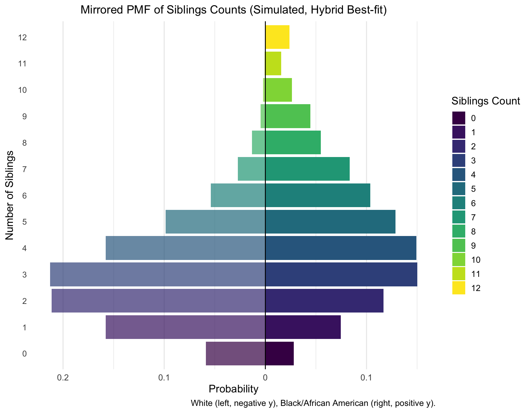

Past versions of unnamed-chunk-21-1.png

Version	Author	Date
b9c32a9	Tina Lasisi	2025-06-18

plot_pmf_mirror(aunts_pmf_hybrid, count_var = "AuntsUncles", category_label = "Aunts/Uncles", cap = 32)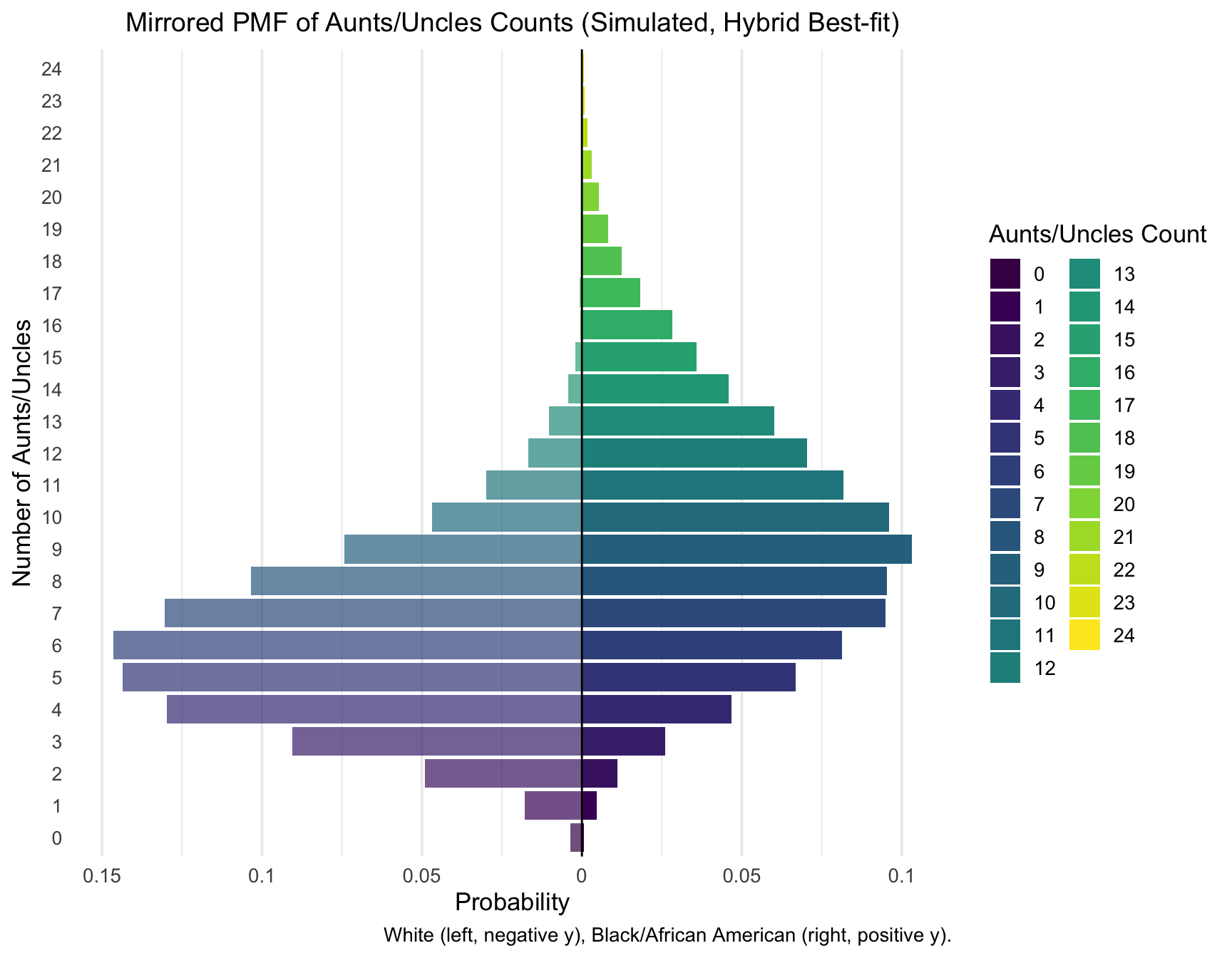

Past versions of unnamed-chunk-21-2.png

Version	Author	Date
b9c32a9	Tina Lasisi	2025-06-18

plot_pmf_mirror(cousins_pmf_hybrid, count_var = "Cousins", category_label = "Cousins", cap = 80)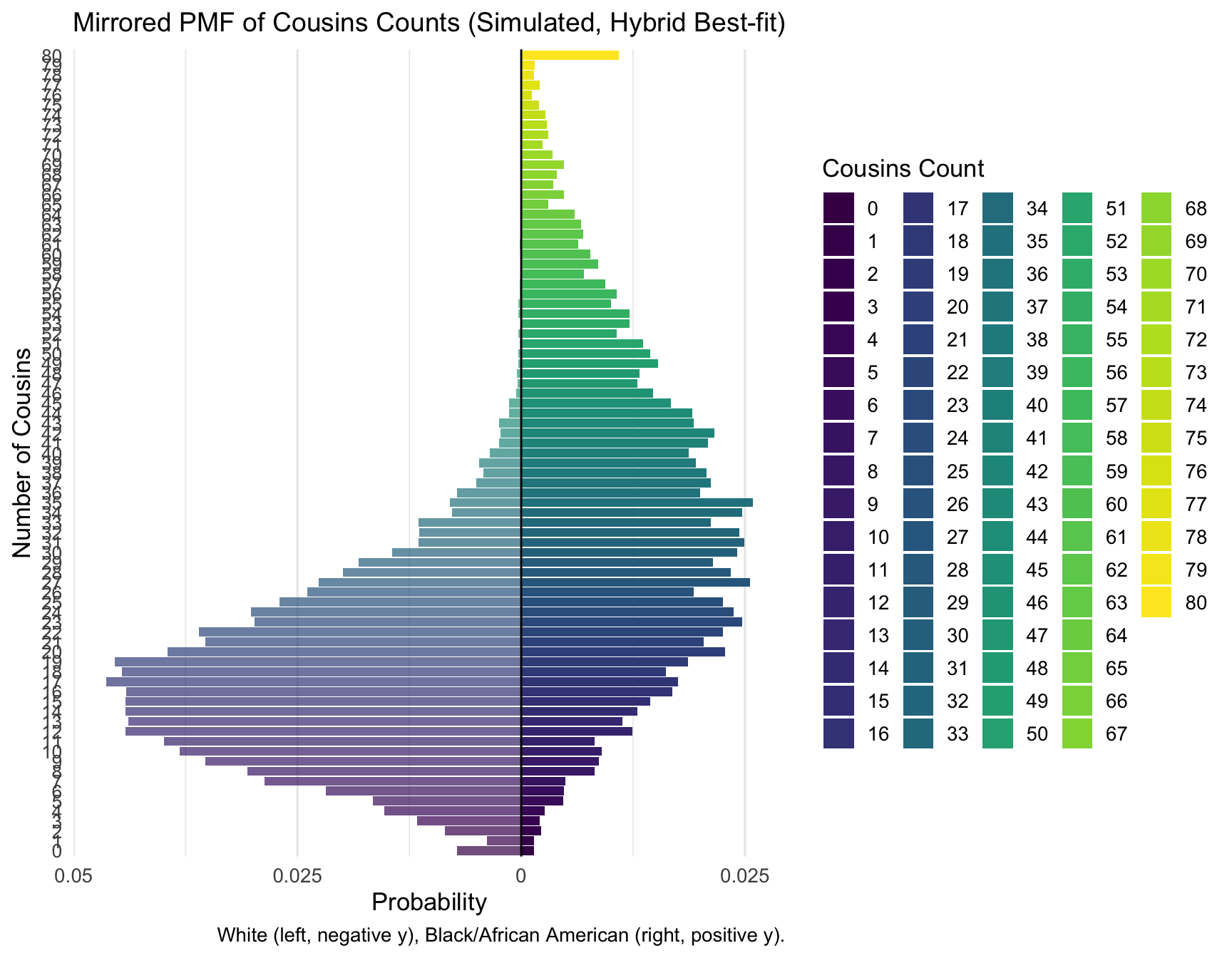

Past versions of unnamed-chunk-21-3.png

Version	Author	Date
b9c32a9	Tina Lasisi	2025-06-18

# Combine hybrid and Poisson baseline sims
compare_means <- bind_rows(hybrid_sim, fixed_poisson_sim) %>%
  group_by(Scenario, RACE) %>%
  summarise(
    mean_sibs = mean(Siblings),
    mean_aunts_uncles = mean(AuntsUncles),
    mean_cousins = mean(Cousins),
    mean_total = mean(TotalKin),
    .groups = "drop"
  )

knitr::kable(compare_means, digits = 2,
  caption = "Mean close-kin counts: hybrid best-fit vs. fixed Poisson baseline (siblings=1.5, fertility=2.5)"
)

Mean close-kin counts: hybrid best-fit vs. fixed Poisson baseline (siblings=1.5, fertility=2.5)

Scenario	RACE	mean_sibs	mean_aunts_uncles	mean_cousins	mean_total
Fixed Poisson (1.5/2.5)	Black/African American	1.49	3.00	7.52	18.01
Fixed Poisson (1.5/2.5)	White	1.52	3.01	7.53	18.06
Hybrid best-fit (ZINB fert)	Black/African American	4.77	9.52	35.19	55.48
Hybrid best-fit (ZINB fert)	White	3.04	6.15	17.81	33.01

summarize_kin <- function(df) {
  df %>%
    tidyr::pivot_longer(
      c(Siblings, AuntsUncles, Cousins, TotalKin),
      names_to = "Relative",
      values_to = "Count"
    ) %>%
    group_by(RACE, Relative) %>%
    summarise(
      min    = min(Count),
      q1     = quantile(Count, 0.25),
      mean   = mean(Count),
      median = median(Count),
      q3     = quantile(Count, 0.75),
      max    = max(Count),
      .groups = "drop"
    )
}

hybrid_summary <- summarize_kin(hybrid_sim) %>%
  rename_with(~ paste0("hybrid_", .), c("min","q1","mean","median","q3","max"))

poisson_summary <- summarize_kin(fixed_poisson_sim) %>%
  rename_with(~ paste0("poisson_", .), c("min","q1","mean","median","q3","max"))

library(dplyr)

side_by_side <- hybrid_summary %>%
  left_join(poisson_summary, by = c("RACE", "Relative"))

knitr::kable(
  side_by_side,
  digits = 2,
  caption = "Summary statistics for simulated kin counts: Hybrid (NB/ZINB) vs. Fixed Poisson baseline"
)

Summary statistics for simulated kin counts: Hybrid (NB/ZINB) vs. Fixed Poisson baseline

RACE	Relative	hybrid_min	hybrid_q1	hybrid_mean	hybrid_median	hybrid_q3	hybrid_max	poisson_min	poisson_q1	poisson_mean	poisson_median	poisson_q3	poisson_max
Black/African American	AuntsUncles	0	7	9.52	9.0	12	24	0	2	3.00	3	4	11
Black/African American	Cousins	0	23	35.19	34.0	46	117	0	4	7.52	7	11	36
Black/African American	Siblings	0	3	4.77	4.0	6	12	0	1	1.49	1	2	8
Black/African American	TotalKin	7	40	55.48	53.5	69	151	6	13	18.01	17	22	55
White	AuntsUncles	0	4	6.15	6.0	8	20	0	2	3.01	3	4	10
White	Cousins	0	11	17.81	17.0	23	61	0	4	7.53	7	11	35
White	Siblings	0	2	3.04	3.0	4	12	0	1	1.52	1	2	8
White	TotalKin	6	25	33.01	32.0	40	87	6	13	18.06	17	22	52

library(ggplot2)

# Create comparison_long for plotting (check if Scenario exists first)
comparison_long <- bind_rows(hybrid_sim, fixed_poisson_sim) %>%
  tidyr::pivot_longer(
    cols = c(Siblings, AuntsUncles, Cousins, TotalKin),
    names_to = "RelativeType",
    values_to = "Count"
  ) %>%
  mutate(
    Scenario = factor(Scenario, levels = c("Fixed Poisson (1.5/2.5)", "Hybrid best-fit (ZINB fert)")),
    RelativeType = factor(RelativeType, levels = c("Siblings", "AuntsUncles", "Cousins", "TotalKin"),
                         labels = c("Siblings", "Aunts/Uncles", "Cousins", "Total Kin"))
  )

# Function to plot each relative type separately (with free y-axis)
plot_kin_box <- function(rel_type) {
  ggplot(comparison_long %>% filter(RelativeType == rel_type),
         aes(x = Scenario, y = Count, fill = RACE)) +
    geom_boxplot(outlier.size = .3, width = 0.7, alpha = 0.8, position = position_dodge(width = 0.7)) +
    stat_summary(
      fun = mean, geom = "point", shape = 21, size = 1.7,
      aes(group = RACE), color = "black", fill = "white",
      position = position_dodge(width = 0.7)
    ) +
    scale_fill_viridis_d(option = "D") +
    labs(
      title = paste("Distribution of", rel_type),
      x = "Simulation scenario",
      y = "Count",
      fill = "Race"
    ) +
    theme_minimal(base_size = 13) +
    theme(
      legend.position = "top",
      panel.grid.major.x = element_blank(),
      strip.text = element_text(size = 12),
      axis.text.x = element_text(angle = 15, vjust = 1, hjust = 1)
    )
}

# Now, print all four plots (one for each relative type)
plot_kin_box("Siblings")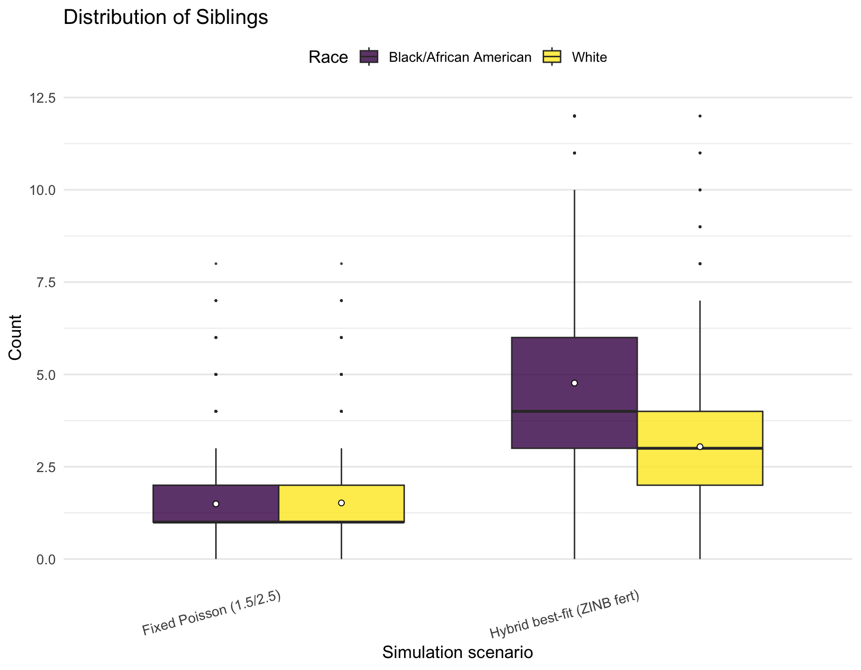

Past versions of unnamed-chunk-26-1.png

Version	Author	Date
b9c32a9	Tina Lasisi	2025-06-18

plot_kin_box("Aunts/Uncles")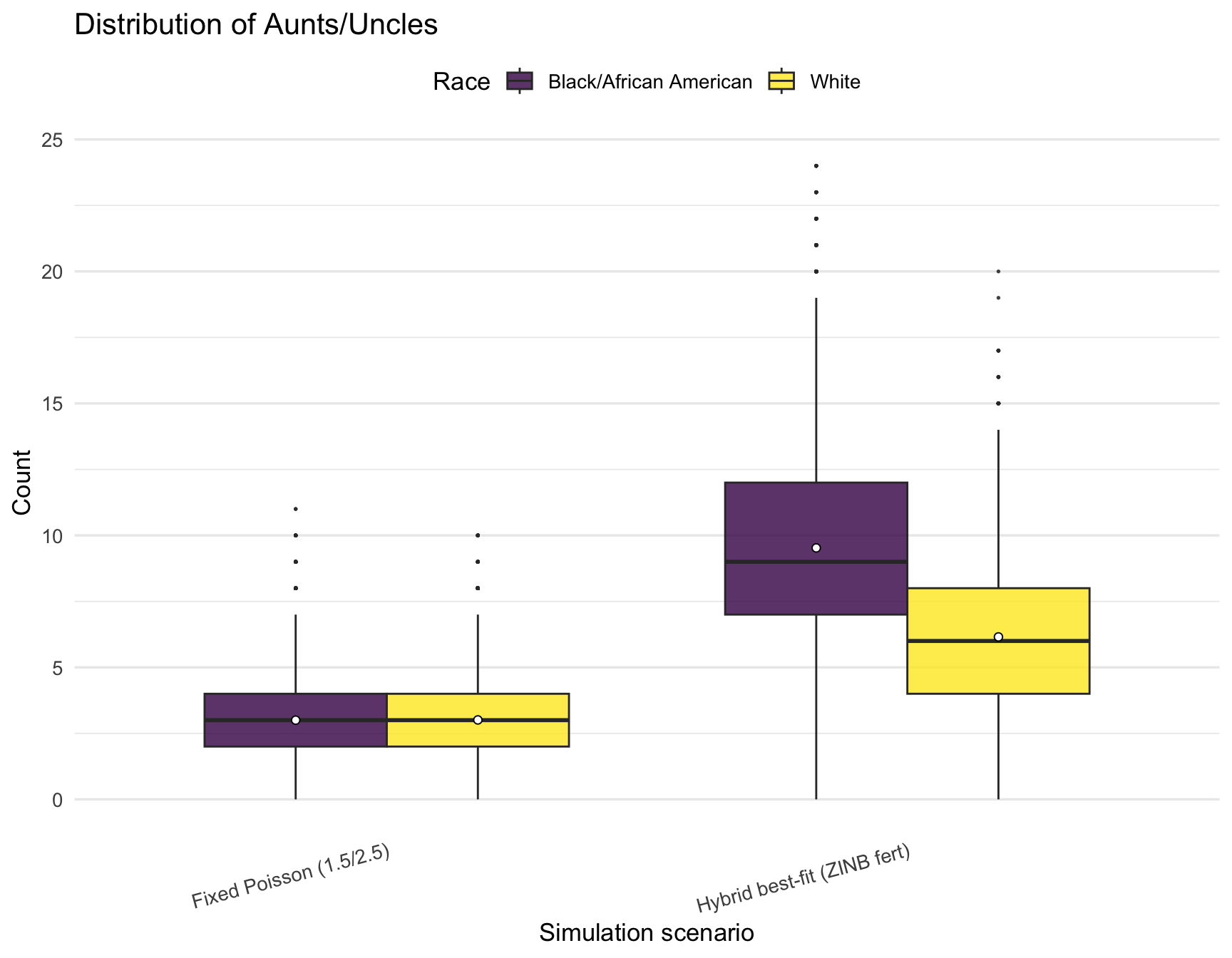

Past versions of unnamed-chunk-26-2.png

Version	Author	Date
b9c32a9	Tina Lasisi	2025-06-18

plot_kin_box("Cousins")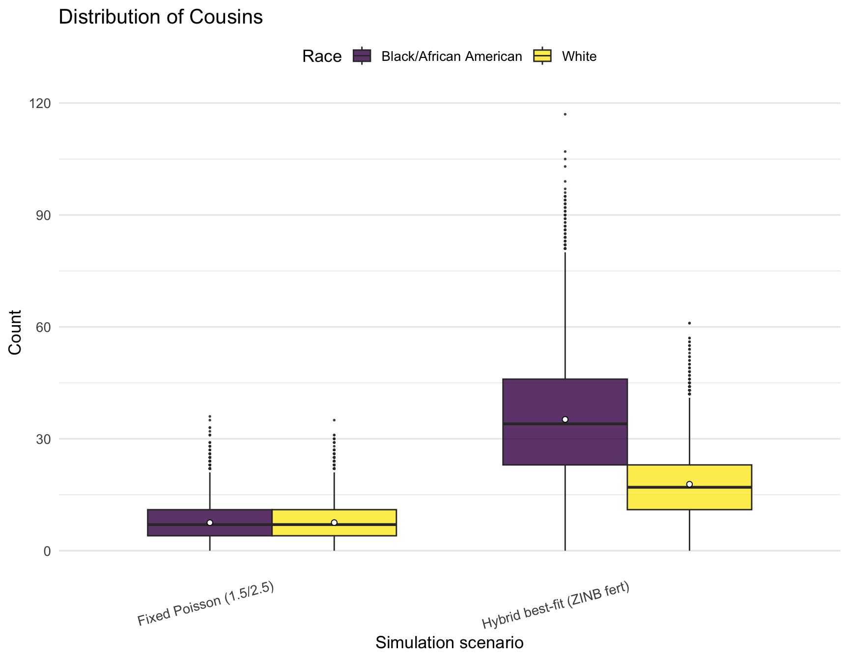

Past versions of unnamed-chunk-26-3.png

Version	Author	Date
b9c32a9	Tina Lasisi	2025-06-18

plot_kin_box("Total Kin")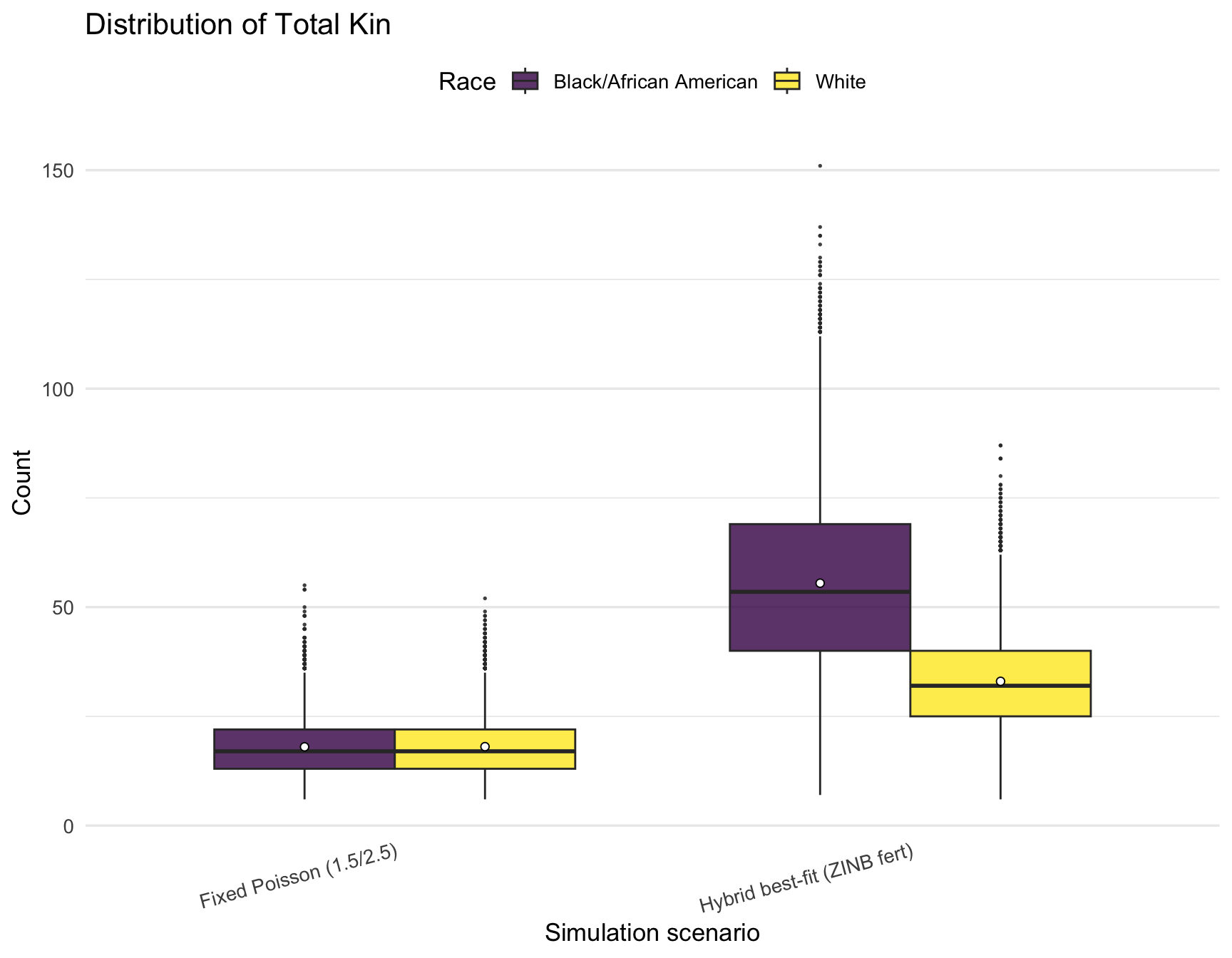

Past versions of unnamed-chunk-26-4.png

Version	Author	Date
b9c32a9	Tina Lasisi	2025-06-18

# Make sure Scenario is present and named correctly
names(hybrid_sim)

 [1] "RACE"         "sib_Model"    "sib_mu"       "sib_size"     "sib_pi0"     
 [6] "sib_AIC"      "fert_Model"   "fert_mu"      "fert_size"    "fert_pi0"    
[11] "fert_AIC"     "Scenario"     "Siblings"     "AuntsUncles"  "Cousins"     
[16] "Parents"      "Grandparents" "TotalKin"    

names(fixed_poisson_sim)

 [1] "RACE"         "sib_Model"    "sib_mu"       "sib_size"     "sib_pi0"     
 [6] "fert_Model"   "fert_mu"      "fert_size"    "fert_pi0"     "Scenario"    
[11] "Siblings"     "AuntsUncles"  "Cousins"      "Parents"      "Grandparents"
[16] "TotalKin"    

# Filter for just TotalKin before running the regression
comparison_total <- bind_rows(
  hybrid_sim %>% mutate(Scenario = "Hybrid best-fit (ZINB fert)"),
  fixed_poisson_sim %>% mutate(Scenario = "Fixed Poisson (1.5/2.5)")
) %>%
  mutate(
    Scenario = factor(Scenario, levels = c("Fixed Poisson (1.5/2.5)", "Hybrid best-fit (ZINB fert)")),
    RACE = factor(RACE, levels = c("White", "Black/African American"))
  )

# Now run the regression on TotalKin
lm_hybrid_vs_pois <- lm(TotalKin ~ Scenario * RACE, data = comparison_total)
summary(lm_hybrid_vs_pois)

Call:
lm(formula = TotalKin ~ Scenario * RACE, data = comparison_total)

Residuals:
    Min      1Q  Median      3Q     Max 
-48.479  -7.011  -1.011   5.989  95.521 

Coefficients:
                                                               Estimate
(Intercept)                                                     18.0622
ScenarioHybrid best-fit (ZINB fert)                             14.9490
RACEBlack/African American                                      -0.0507
ScenarioHybrid best-fit (ZINB fert):RACEBlack/African American  22.5188
                                                               Std. Error
(Intercept)                                                        0.1268
ScenarioHybrid best-fit (ZINB fert)                                0.1794
RACEBlack/African American                                         0.1794
ScenarioHybrid best-fit (ZINB fert):RACEBlack/African American     0.2537
                                                               t value Pr(>|t|)
(Intercept)                                                    142.415   <2e-16
ScenarioHybrid best-fit (ZINB fert)                             83.345   <2e-16
RACEBlack/African American                                      -0.283    0.777
ScenarioHybrid best-fit (ZINB fert):RACEBlack/African American  88.777   <2e-16
                                                                  
(Intercept)                                                    ***
ScenarioHybrid best-fit (ZINB fert)                            ***
RACEBlack/African American                                        
ScenarioHybrid best-fit (ZINB fert):RACEBlack/African American ***
---
Signif. codes:  0 '***' 0.001 '**' 0.01 '*' 0.05 '.' 0.1 ' ' 1

Residual standard error: 12.68 on 39996 degrees of freedom
Multiple R-squared:  0.5935,    Adjusted R-squared:  0.5935 
F-statistic: 1.946e+04 on 3 and 39996 DF,  p-value: < 2.2e-16

knitr::kable(broom::tidy(lm_hybrid_vs_pois), digits = 3,
             caption = "Regression coefficients: effect of simulation scenario (Hybrid vs Poisson) on total close relatives")

Regression coefficients: effect of simulation scenario (Hybrid vs Poisson) on total close relatives

term	estimate	std.error	statistic	p.value
(Intercept)	18.062	0.127	142.415	0.000
ScenarioHybrid best-fit (ZINB fert)	14.949	0.179	83.345	0.000
RACEBlack/African American	-0.051	0.179	-0.283	0.777
ScenarioHybrid best-fit (ZINB fert):RACEBlack/African American	22.519	0.254	88.777	0.000

Session information

sessionInfo()

R version 4.5.0 (2025-04-11)
Platform: aarch64-apple-darwin20
Running under: macOS Sequoia 15.5

Matrix products: default
BLAS:   /Library/Frameworks/R.framework/Versions/4.5-arm64/Resources/lib/libRblas.0.dylib 
LAPACK: /Library/Frameworks/R.framework/Versions/4.5-arm64/Resources/lib/libRlapack.dylib;  LAPACK version 3.12.1

locale:
[1] en_US.UTF-8/en_US.UTF-8/en_US.UTF-8/C/en_US.UTF-8/en_US.UTF-8

time zone: America/Detroit
tzcode source: internal

attached base packages:
[1] stats     graphics  grDevices utils     datasets  methods   base     

other attached packages:
 [1] viridisLite_0.4.2 broom_1.0.8       ggplot2_3.5.2     purrr_1.0.4      
 [5] knitr_1.50        pscl_1.5.9        MASS_7.3-65       readr_2.1.5      
 [9] tidyr_1.3.1       dplyr_1.1.4       workflowr_1.7.1  

loaded via a namespace (and not attached):
 [1] sass_0.4.10        utf8_1.2.5         generics_0.1.4     stringi_1.8.7     
 [5] hms_1.1.3          digest_0.6.37      magrittr_2.0.3     RColorBrewer_1.1-3
 [9] grid_4.5.0         evaluate_1.0.3     fastmap_1.2.0      rprojroot_2.0.4   
[13] jsonlite_2.0.0     processx_3.8.6     whisker_0.4.1      backports_1.5.0   
[17] ps_1.9.1           promises_1.3.3     httr_1.4.7         scales_1.4.0      
[21] jquerylib_0.1.4    cli_3.6.5          rlang_1.1.6        crayon_1.5.3      
[25] bit64_4.6.0-1      withr_3.0.2        cachem_1.1.0       yaml_2.3.10       
[29] tools_4.5.0        parallel_4.5.0     tzdb_0.5.0         httpuv_1.6.16     
[33] vctrs_0.6.5        R6_2.6.1           lifecycle_1.0.4    git2r_0.36.2      
[37] stringr_1.5.1      fs_1.6.6           bit_4.6.0          vroom_1.6.5       
[41] pkgconfig_2.0.3    callr_3.7.6        gtable_0.3.6       pillar_1.10.2     
[45] bslib_0.9.0        later_1.4.2        glue_1.8.0         Rcpp_1.0.14       
[49] xfun_0.52          tibble_3.3.0       tidyselect_1.2.1   dichromat_2.0-0.1 
[53] rstudioapi_0.17.1  farver_2.1.2       htmltools_0.5.8.1  labeling_0.4.3    
[57] rmarkdown_2.29     compiler_4.5.0     getPass_0.2-4