Family size findability
Junhui He and Tina Lasisi
2025-06-22 15:46:07
Last updated: 2025-06-22
Checks: 7 0
Knit directory: PODFRIDGE/
This reproducible R Markdown analysis was created with workflowr (version 1.7.1). The Checks tab describes the reproducibility checks that were applied when the results were created. The Past versions tab lists the development history.
Great! Since the R Markdown file has been committed to the Git repository, you know the exact version of the code that produced these results.
Great job! The global environment was empty. Objects defined in the global environment can affect the analysis in your R Markdown file in unknown ways. For reproduciblity it’s best to always run the code in an empty environment.
The command set.seed(20230302) was run prior to running
the code in the R Markdown file. Setting a seed ensures that any results
that rely on randomness, e.g. subsampling or permutations, are
reproducible.
Great job! Recording the operating system, R version, and package versions is critical for reproducibility.
Nice! There were no cached chunks for this analysis, so you can be confident that you successfully produced the results during this run.
Great job! Using relative paths to the files within your workflowr project makes it easier to run your code on other machines.
Great! You are using Git for version control. Tracking code development and connecting the code version to the results is critical for reproducibility.
The results in this page were generated with repository version c96e544. See the Past versions tab to see a history of the changes made to the R Markdown and HTML files.
Note that you need to be careful to ensure that all relevant files for
the analysis have been committed to Git prior to generating the results
(you can use wflow_publish or
wflow_git_commit). workflowr only checks the R Markdown
file, but you know if there are other scripts or data files that it
depends on. Below is the status of the Git repository when the results
were generated:
Ignored files:
    Ignored:    .DS_Store
    Ignored:    .Rhistory
    Ignored:    .Rproj.user/
    Ignored:    analysis/.DS_Store
    Ignored:    code/.DS_Store
    Ignored:    output/.DS_Store

Untracked files:
    Untracked:  data/Murphy_combined_data.csv

Unstaged changes:
    Modified:   analysis/racial_proportion.Rmd
    Modified:   analysis/regression.Rmd
    Modified:   data/final_CODIS_data.csv
Note that any generated files, e.g. HTML, png, CSS, etc., are not included in this status report because it is ok for generated content to have uncommitted changes.
These are the previous versions of the repository in which changes were
made to the R Markdown
(analysis/family_size_findability.Rmd) and HTML
(docs/family_size_findability.html) files. If you’ve
configured a remote Git repository (see ?wflow_git_remote),
click on the hyperlinks in the table below to view the files as they
were in that past version.
| File | Version | Author | Date | Message |
|---|---|---|---|---|
| Rmd | 85a529f | Tina Lasisi | 2025-06-04 | Add ZINB family size analysis with Erlich comparison |
| html | 85a529f | Tina Lasisi | 2025-06-04 | Add ZINB family size analysis with Erlich comparison |
| html | 1b48bf1 | Junhui He | 2025-06-03 | Build site. |
| Rmd | e3bbbd9 | Junhui He | 2025-06-03 | family size simulator and cousin-in-database probability |
| html | 9fc81c2 | Junhui He | 2025-06-03 | Build site. |
| Rmd | d1eff03 | Junhui He | 2025-06-03 | family size simulator and cousin-in-database probability |
1. Introduction
We aim to clarify the probability of finding at least one cousin in a database, given the family structure in the PODFRIDGE project. This probability depends on two key factors: the number of relatives—determined by the family size (number of children per family) distribution—and the database coverage, which is the proportion of individuals in the database relative to the total population.
Erlich’s earlier paper modeled the family size distribution using a Poisson distribution, a common approach in many genetic studies. However, this assumption doesn’t accurately capture real-world family sizes, which often show overdispersion and an excess of zeros (i.e., families with no children).
In this report, we simulate the family size distribution using a Zero-Inflated Negative Binomial (ZINB) distribution, which better reflects real-world data than the Poisson model. We then calculate the probability of finding at least one cousin in the database based on the simulated family sizes and different levels of database coverage.
2. Methods
2.1. Zero-Inflated Negative Binomial (ZINB) Distribution
Based on the empirical data from the US, we find that the distribution of family size is better modeled as a Zero-Inflated Negative Binomial (ZINB) distribution. The ZINB distribution is a more realistic family size distribution, as it accounts for the excess zeros (families with no children) and the overdispersion often observed in family size data.
The Zero-Inflated Negative Binomial (ZINB) distribution is a statistical model that combines a negative binomial distribution with an additional process that generates excess zeros. It is characterized by three parameters: the zero-inflated probability \(p\), the mean number \(\mu\) and the size \(s\) of the negative binomial distribution, denoted by \(\text{ZINB}(p, s, \mu) = p\delta_0 + (1-p)\text{NB}(s,\mu)\). The average family size is \((1-p)\mu\). Based on empirical data, we set the parameters to \(p=0.1, ~ s=3, ~ \mu = 3\).
2.2. Calculating the Number of Relatives
In this report, we only consider the relatives whose generation difference between the individual and the relative is less than or equal to 1. Therefore, the first-degree relatives include parents, siblings, and children; the second-degree relatives include aunts, uncles, nephews, nieces, and half-siblings; and the third-degree relatives include first cousins. The number of relatives is calculated based on the family size distribution simulated by the ZINB distribution. For now, the number of half-siblings is set to 0.
Specifically, if one couple is known as the ancestor couple of the individual, this couple has at least one child, and the number of children is simulated from the ZINB distribution conditional on at least one child. For simplicity, we assume that \(X\) follows a ZINB distribution and \(Y\) follows a ZINB distribution conditional on at least one child minus one.
The number of first-degree relatives is given by \(2+Y+X\). The number of second-degree relatives is given by \(4 + \sum_{i=1}^2Y_i + \sum_{i=1}^{Y}X_i\). The number of third-degree relatives is given by \(\sum_{i=1}^{\sum_{j=1}^2 Y_j} X_i\).
Remark: For simplicity, sometimes we approximate the number of second-degree relatives as \(4 + 2Y + YX\), and the number of third-degree relatives as \(2YX\).
2.3 The Probability of Finding at Least One Cousin in the Database
The number of cousins is simulated from the ZINB distribution as above. The simulated data is denoted as \(\{r_k\}_{k=1}^n\), where \(n\) is the number of simulations. For each simulated number of cousins \(r_k\), we assume that the number of cousins found in the database follows a binomial distribution with parameters \(r_k\) and the coverage of the database \(c\), denoted as \(\text{Binomial}(r_k, c)\). The probability of finding at least one cousin in the database is therefore \(1-(1-c)^{r_k}\). The expected probability across all simulations is given by \(\frac{1}{n}\sum_{k=1}^n (1-(1-c)^{r_k})\).
3. Results
3.1. Family Size Simulation
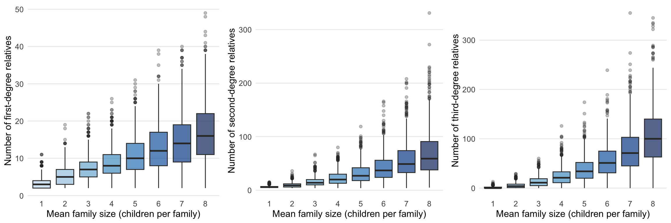
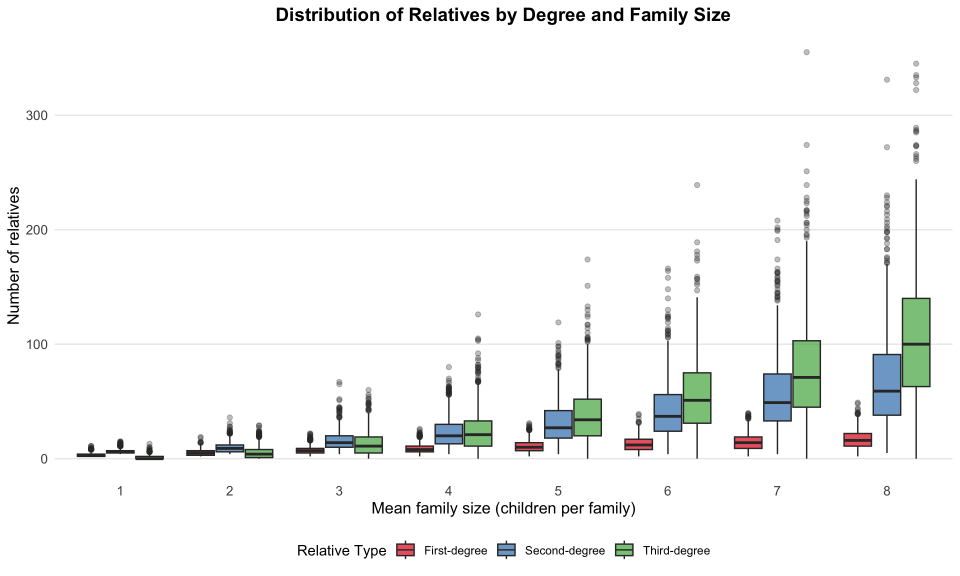
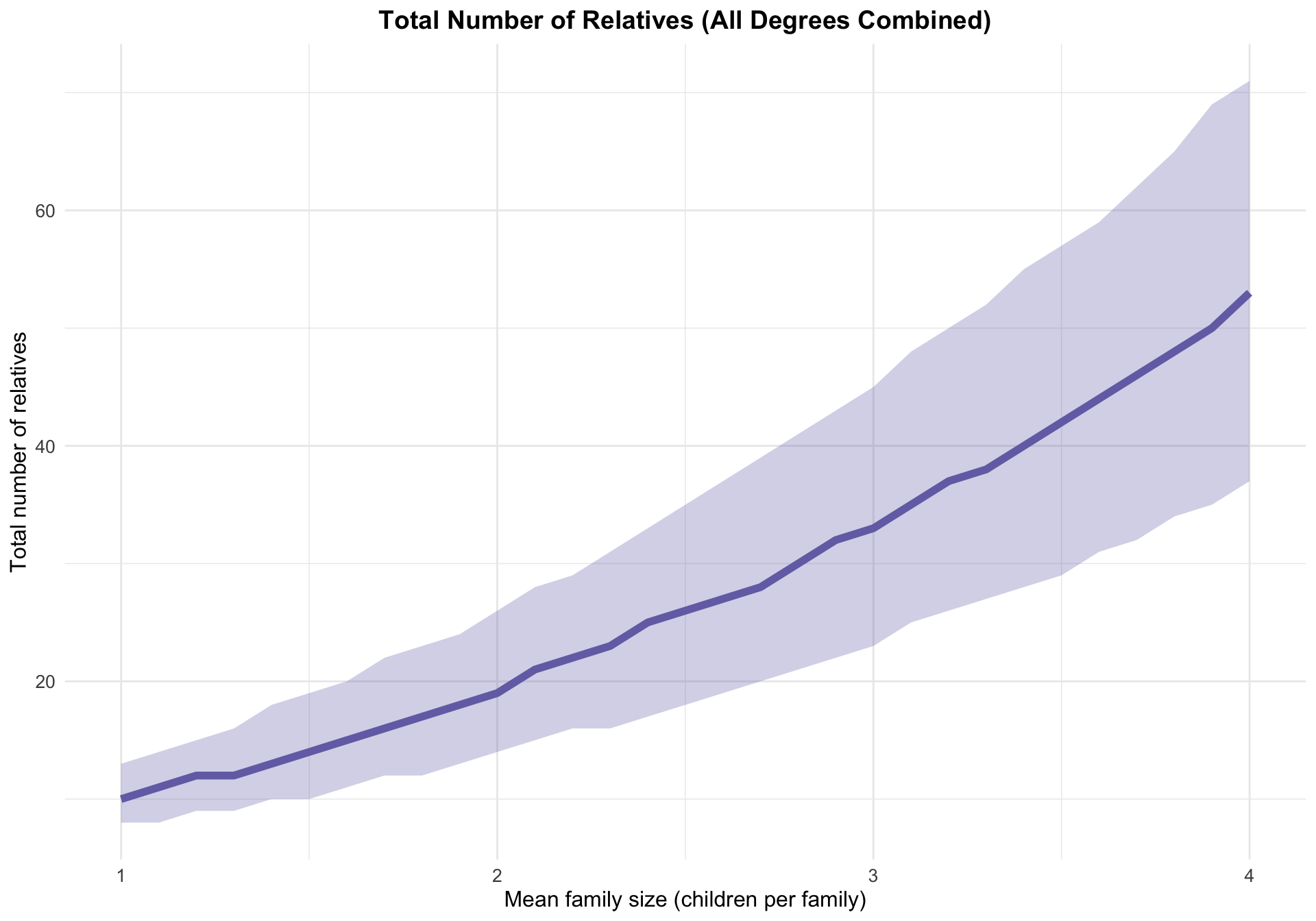
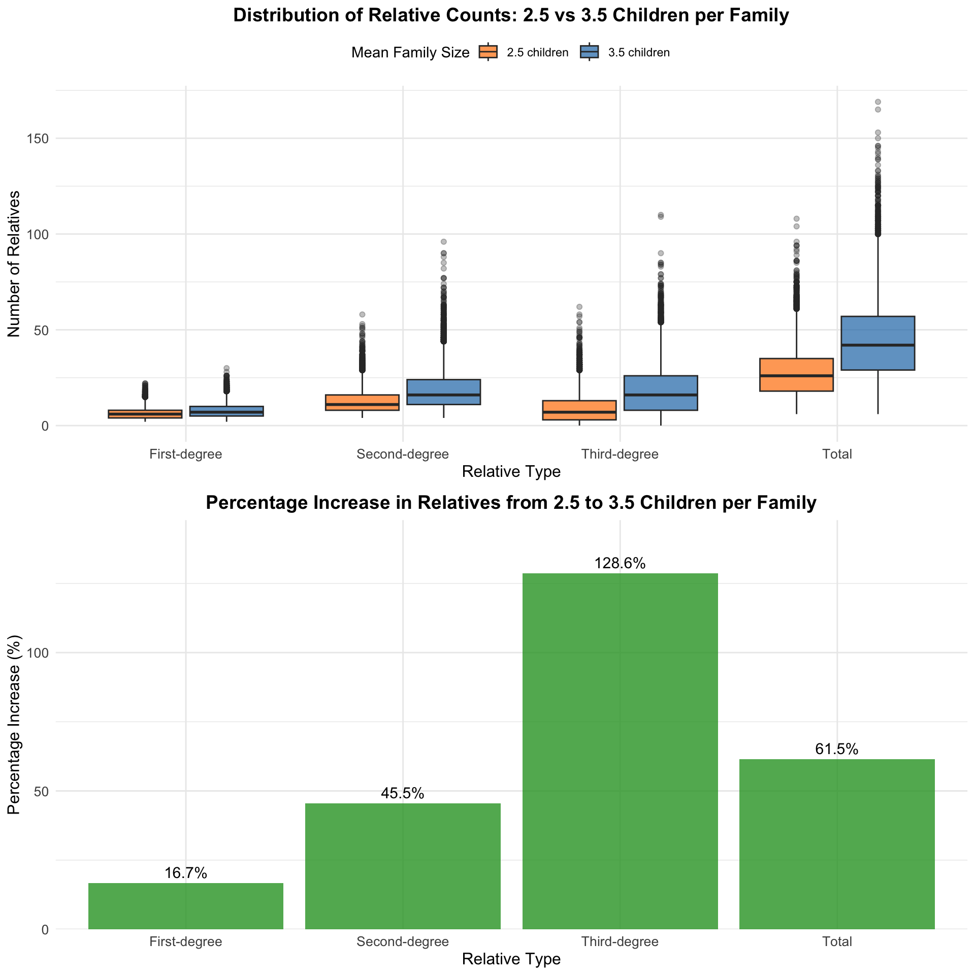
We explore the distribution of first-, second-, and third-degree relatives as family size increases in the simulation. Specifically, we fix the zero-inflated probability \(p=0.1\), and the size \(s=3\) of the ZINB distribution, and vary the mean number \(\mu\) from 1 to 8. The simulation is run for 1000 times, and the distribution of relatives is calculated for each mean family size. The boxplots show that as the mean family size increases, the number of first-degree, second-degree, and third-degree relatives also increases. This is expected, as larger families tend to have more relatives.
| Version | Author | Date |
|---|---|---|
| 85a529f | Tina Lasisi | 2025-06-04 |
| Version | Author | Date |
|---|---|---|
| 85a529f | Tina Lasisi | 2025-06-04 |
| Version | Author | Date |
|---|---|---|
| 85a529f | Tina Lasisi | 2025-06-04 |
| Version | Author | Date |
|---|---|---|
| 85a529f | Tina Lasisi | 2025-06-04 |
| Version | Author | Date |
|---|---|---|
| 85a529f | Tina Lasisi | 2025-06-04 |
3.2. Relationship between cousin-in-database probability and average family size
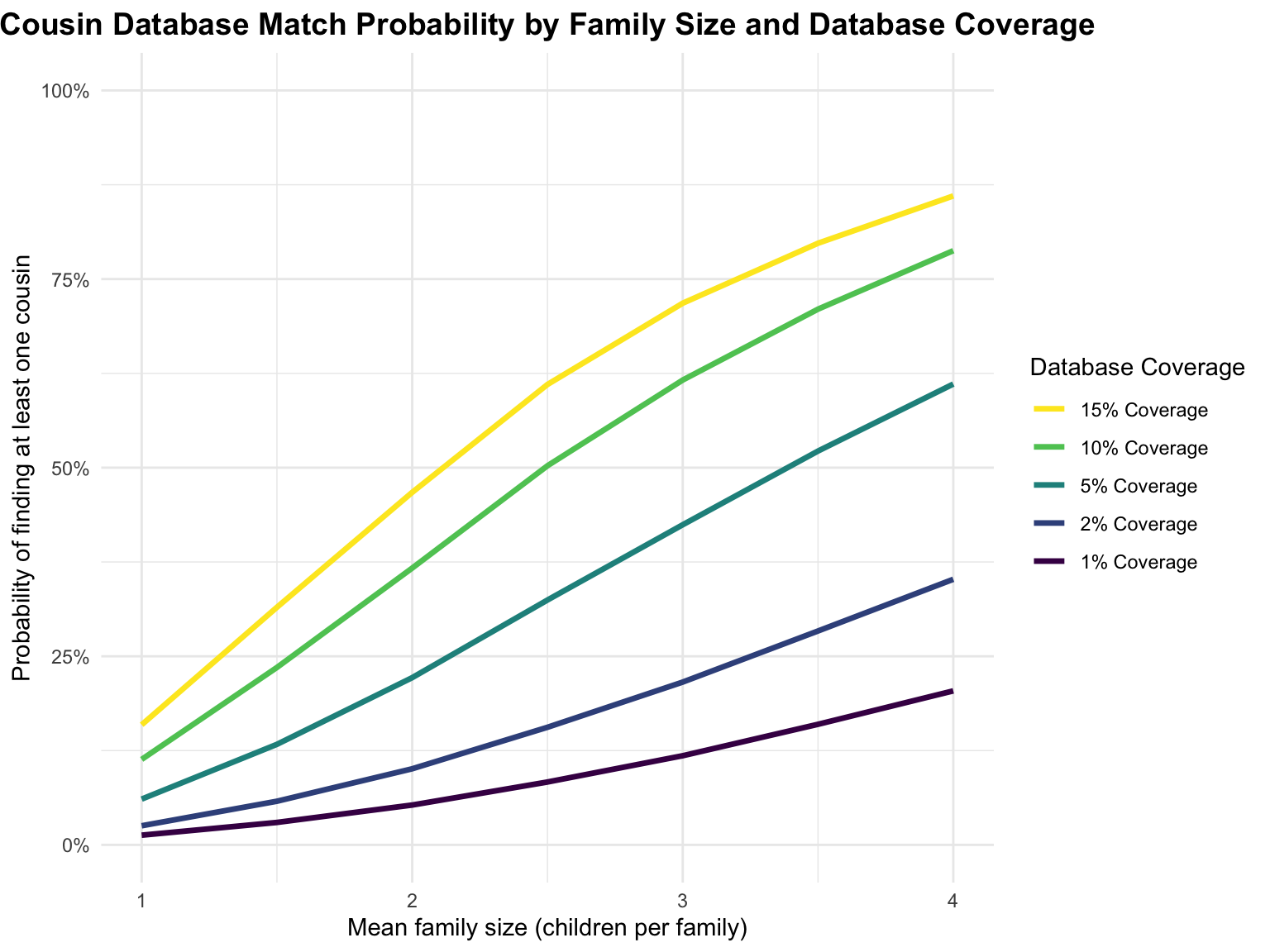
In this section, we explore the relationship between family size and the probability of finding at least one cousin in a database. We simulate family sizes using the ZINB distribution and calculate the probability of finding at least one cousin in a database with varying coverages (e.g., 10%, 30%, 50%). For the ZINB distribution, we set the parameters as follows: zero-inflated probability \(p=0.1\), size \(s=3\), and mean number \(\mu\) varying from 1 to 8. The simulation is run for 1000 times.
We draw a plot for visualizing the relationship between family size and cousin-in-database probability across the chosen database coverages. This plot illustrates that as the mean family size increases, the probability of finding at least one cousin in the database also increases. This is because larger families tend to have more cousins, which increases the chances of finding at least one cousin in a database with a given coverage. In addition, we observe that the probability of finding at least one cousin in the database increases with higher database coverage. This is because a higher coverage means that more individuals are included in the database.
4. Comparison: Erlich Original vs ZINB Family Size Model
To understand how realistic family size distributions affect long-range familial search probabilities, we compare Erlich et al.’s original model with our Zero-Inflated Negative Binomial (ZINB) approach. Both models aim to predict the probability of finding genetic relatives in databases of varying sizes.
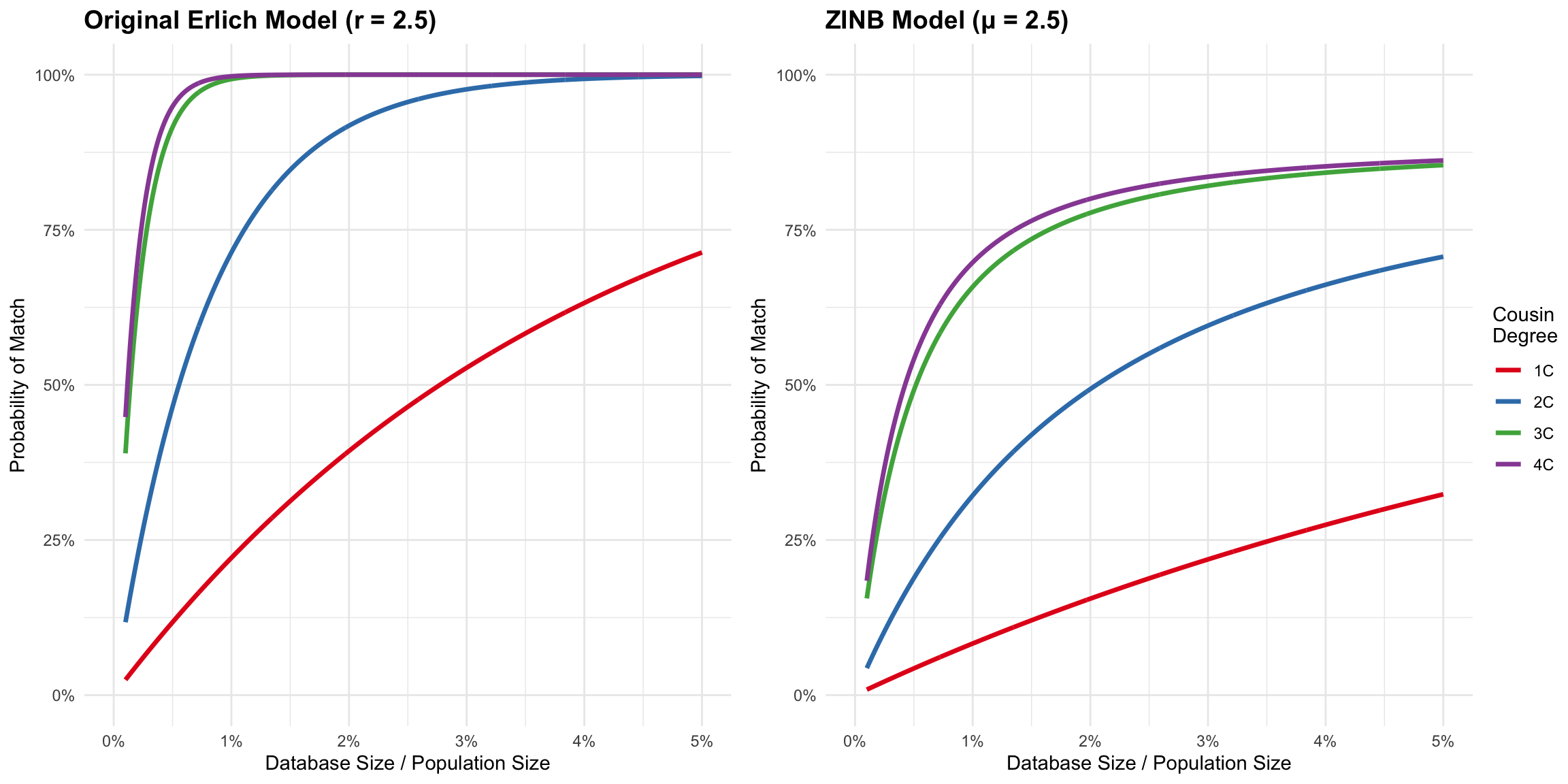
Direct Comparison: Original Erlich (r=2.5) vs ZINB (μ=2.5)
The figure below shows a side-by-side comparison of the two models, both using a mean family size of 2.5 children per couple:
| Version | Author | Date |
|---|---|---|
| 85a529f | Tina Lasisi | 2025-06-04 |
The comparison reveals several key differences:
Lower probabilities across all cousin degrees: The ZINB model consistently predicts lower probabilities of finding relatives compared to Erlich’s model.
Zero inflation impact: With 10% of families having no children in the ZINB model, many genealogical lines terminate, reducing the overall number of cousins.
Variance effects: The ZINB distribution’s higher variance means some families have many relatives while others have very few, creating a more realistic but less predictable pattern.
Sensitivity Analysis: Mean Family Size from 1.5 to 4.0
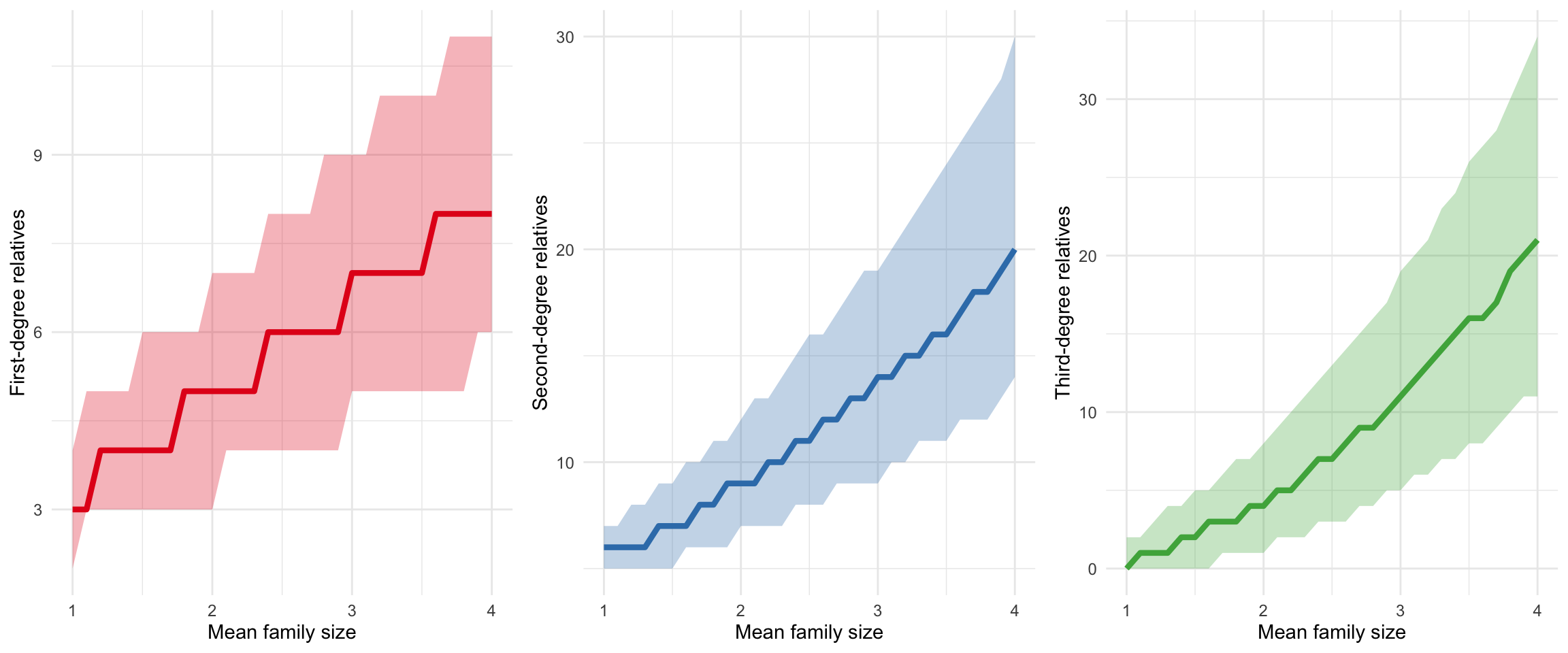
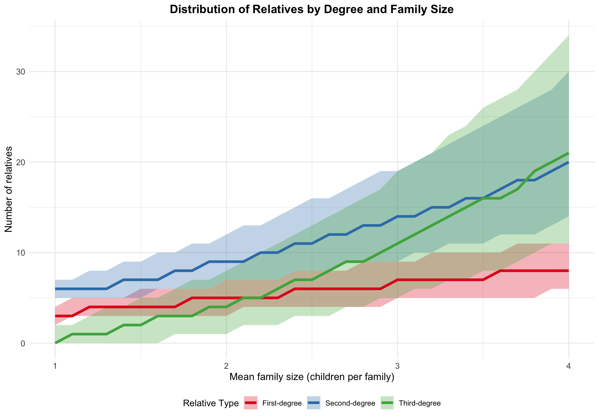
To understand how mean family size affects these probabilities, we examined a range of values from 1.5 to 4.0 children per family:
Warning: Removed 4 rows containing missing values or values outside the scale range
(`geom_text()`).
Removed 4 rows containing missing values or values outside the scale range
(`geom_text()`).
Removed 4 rows containing missing values or values outside the scale range
(`geom_text()`).
Removed 4 rows containing missing values or values outside the scale range
(`geom_text()`).
Removed 4 rows containing missing values or values outside the scale range
(`geom_text()`).
Removed 4 rows containing missing values or values outside the scale range
(`geom_text()`).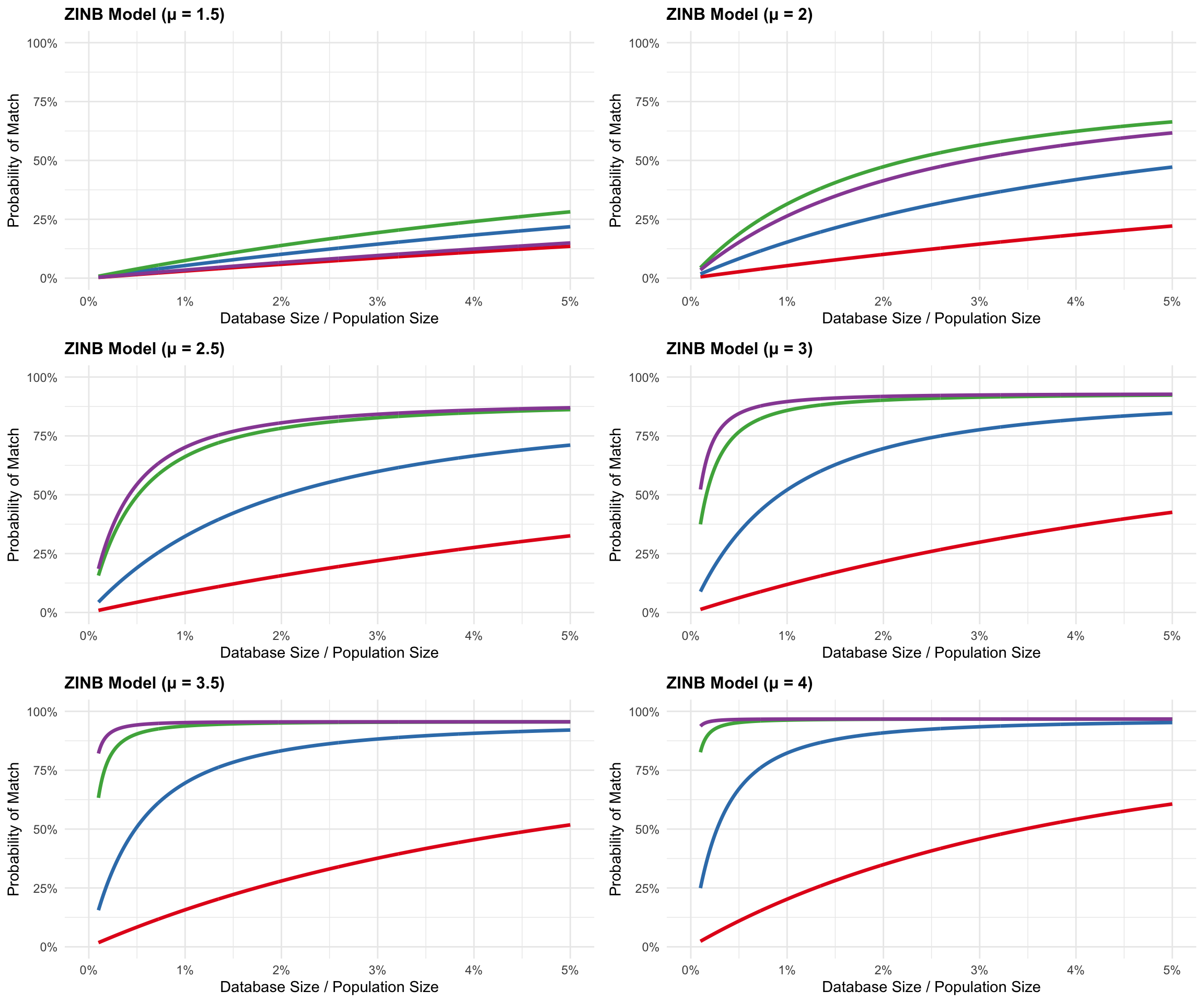
| Version | Author | Date |
|---|---|---|
| 85a529f | Tina Lasisi | 2025-06-04 |
Key Findings
The ZINB model reveals several important insights about familial search probabilities:
Non-linear scaling: The probability of finding relatives doesn’t scale linearly with mean family size. The difference between μ=1.5 and μ=2.0 is much smaller than between μ=3.5 and μ=4.0.
Database coverage threshold: For smaller family sizes (μ < 2), even large databases (5% of population) have limited success in finding distant cousins.
Fourth cousin saturation: With larger family sizes (μ ≥ 3), the probability of finding fourth cousins approaches certainty even with modest database coverage (2-3%).
Real-world implications: Most developed countries have fertility rates between 1.5-2.5, suggesting that the lower probability curves are more representative of actual genealogical networks.
These results suggest that Erlich et al.’s original estimates may be overly optimistic for populations with realistic family size distributions, particularly when accounting for childless couples and the high variance in family sizes observed in real populations.
5. Conclusion
The family size distribution is better modeled as a Zero-Inflated Negative Binomial (ZINB) distribution than a Poisson distribution, which accounts for the excess zeros and overdispersion often observed in realistic family size data.
The number of relatives increases with the mean family size,.
The probability of finding at least one cousin in a database increases with both the mean family size and the coverage of the database. Larger families tend to have more cousins, and higher database coverage means more individuals are included.
R version 4.3.1 (2023-06-16)
Platform: aarch64-apple-darwin20 (64-bit)
Running under: macOS 15.5

Matrix products: default
BLAS:   /Library/Frameworks/R.framework/Versions/4.3-arm64/Resources/lib/libRblas.0.dylib
LAPACK: /Library/Frameworks/R.framework/Versions/4.3-arm64/Resources/lib/libRlapack.dylib;  LAPACK version 3.11.0

locale:
[1] en_US.UTF-8/en_US.UTF-8/en_US.UTF-8/C/en_US.UTF-8/en_US.UTF-8

time zone: America/Detroit
tzcode source: internal

attached base packages:
[1] stats     graphics  grDevices utils     datasets  methods   base

other attached packages:
[1] RColorBrewer_1.1-3 dplyr_1.1.4        tidyr_1.3.1        ggpubr_0.6.0
[5] ggplot2_3.5.2

loaded via a namespace (and not attached):
 [1] sass_0.4.10       generics_0.1.4    rstatix_0.7.2     stringi_1.8.7
 [5] digest_0.6.37     magrittr_2.0.3    evaluate_1.0.3    grid_4.3.1
 [9] fastmap_1.2.0     rprojroot_2.0.4   workflowr_1.7.1   jsonlite_2.0.0
[13] whisker_0.4.1     backports_1.5.0   Formula_1.2-5     gridExtra_2.3
[17] promises_1.3.3    purrr_1.0.4       scales_1.4.0      textshaping_1.0.1
[21] jquerylib_0.1.4   abind_1.4-8       cli_3.6.5         rlang_1.1.6
[25] cowplot_1.1.3     withr_3.0.2       cachem_1.1.0      yaml_2.3.10
[29] tools_4.3.1       ggsignif_0.6.4    httpuv_1.6.16     broom_1.0.8
[33] vctrs_0.6.5       R6_2.6.1          lifecycle_1.0.4   git2r_0.36.2
[37] stringr_1.5.1     fs_1.6.6          car_3.1-3         ragg_1.4.0
[41] pkgconfig_2.0.3   pillar_1.10.2     bslib_0.9.0       later_1.4.2
[45] gtable_0.3.6      glue_1.8.0        Rcpp_1.0.14       systemfonts_1.2.3
[49] xfun_0.52         tibble_3.2.1      tidyselect_1.2.1  rstudioapi_0.17.1
[53] knitr_1.50        farver_2.1.2      htmltools_0.5.8.1 labeling_0.4.3
[57] rmarkdown_2.29    carData_3.0-5     compiler_4.3.1